Analysis of Travel Choices and Scenarios for Sharing Rides
| |||||||||||||||||||||||||||||||||||||||||||||||||||||||||||||||||||||||||||||||||||||||||||||||||||||||||||||||||||||||||||||||||||||||||||||||||||||||||||||||||||||||||||||||||||||||||||||||||||||||||||||||||||||||||||||||||||||||||||||||||||||||||||||||||||||||||||||||||||||||||||||||||||||||||||||||||||||||||||||||||||||||||||||||||||||||||||||||||||||||||||||||||||||||||||||||||||||||||||||||||||||||||||||||||||||||||||||||||||||||||||||||||||||||||||||||||||||||||||||||||||||||||||||||||||||||||||||||||||||||||||||||||||||||||||||||||||||||||||||||||||||||||||||||||||||||||||||||||||||||||||||||||||||||||||||||||||||||||||||||||||||||||||||||||||||||||||||||||||||||||||||||||||||||||||||||||||||||||||||||||||||||||||||||||||||||||||||||||||||||||||||||||||||||||||||||||
| Scenario | Basis | Data Source | |
|---|---|---|---|
| 1 | Increase cost savings for shared transportation network company (TNC) trips relative to private TNC trips | Dollar per mile | TNC survey findings (Chapter 2) |
| 2 | Reduce travel time penalty for shared TNC trips relative to private TNC trips | Minute per trip | TNC survey findings (Chapter 2) |
| 3 | Increase price differential between private vehicle car trips and all other modes | Dollar per trip | Literature review |
| 4 | (Experimental) Reward shared personal vehicle car trips but not private car trips | Dollar (or points) per trip | App-based carpooling findings (Chapter 3) |
This initial scenario applies only to for-hire and TNC rides, specifically to the price difference between private and shared for-hire or TNC rides. This difference could be influenced through a number of mechanisms, including but not limited to fees (or rebates) on private TNC and for-hire rides. This price difference can be understood on a per-mile or a per-trip basis but is modeled in this research in terms of dollars per mile, in order to control for differences in trip lengths. Price differences apply to individual travelers or traveler parties. The expected effect of such a scenario would be to increase occupancy of TNC trips. This scenario is feasible to implement from a technical perspective and possible to model using the output of the TNC survey research described in chapter 2 (see figure 5).
Unlike scenario 1, this scenario applies to time rather than cost. Under this scenario, shared TNCs would enjoy faster and more reliable travel times. While it is difficult to affect travel times in a consistent way, transportation facilities and policies (e.g., exclusive access to dedicated travel lanes or enforced delay on private TNC trips) could provide mechanisms for improving the relative travel time of shared TNC trips. Another possible mechanism for influencing relative travel time would be for a city to set a limit on the number of private TNC trips that may be underway at a given time through a metering system.2 When private rides are in high demand, users would then have the option to wait for a private ride or skip the "virtual queue" by accepting a shared ride (for which there is no cap). Naturally, this supply-side policy could also have the effect of increasing the cost of private TNC rides, but it is difficult to predict exactly how the private sector would react to such a policy. Whatever the case may be, public agencies would likely require audit authority of TNCs and the ability to penalize violations in order to enforce this mechanism.
Whatever the exact mechanism may be, the expected impact of this scenario is to discourage single-occupancy travel by TNC (or for-hire vehicle). Like scenario 1, it is possible to model the impact of this policy using the output of the TNC survey research described in chapter 1. As with scenario 1, travel time difference is modeled in terms of minutes per mile, in order to control for differences in trip lengths (see figure 7).
Unlike scenarios 1 and 2, this scenario applies to the relative cost of private vehicle trips. It corresponds to mechanisms such as providing all residents of an area a refundable transportation expense allowance and then deducting from this allowance a per-trip fee on non-shared private vehicles crossing into or parking within a specific cordoned area. The fees could function as a fee for all trips and a rebate for verified carpools. The expected effect of such a scenario would be to increase travel by transit, carpool, TNC, and nonmotorized modes. This scenario is feasible to implement from a technical perspective and possible to model using a review of relevant literature.
To use studies of parking and non-parking driving costs as a proxy for this scenario, Shoup offers a useful starting point; the study reviewed seven studies conducted between 1969 and 1991 that analyzed the effect of employer-paid parking on SOV commute rates3. The review found that when employers in the analyzed areas paid for parking, 67 percent of employees drove alone. When employees paid for parking themselves in the same areas, the drive-alone rate dropped to 42 percent. Price elasticity for the various employment sites ranged from -0.08 to -0.23, with a mean of -0.15. This elasticity suggests that reducing the price of parking by 10 percent would increase the number of vehicle trips to work by 1.5 percent. However, elasticity—the ratio of percent change in demand to percent change in price—cannot be calculated if the starting price is zero (e.g., free parking), as any price increase would be one of infinity percent. Therefore, these elasticities were not calculated as logarithmic arc elasticity, but rather as linear arc elasticity (also known as midpoint elasticity). Linear arc elasticity approximates the average elasticity between two points along a demand curve. In this case, the percent change in price is defined as the absolute change in price divided by the average of the before and after prices. Because each case study examined the results of raising parking prices from zero to a market price, the change in market price is equal to the market price, and the average of the two prices (zero and market) is always half the market price.
Concas and Nayak conducted a meta-analysis of parking price elasticity using 25 studies that included in total 169 elasticity variables. This review found elasticity values -6.22 to zero, with a mean value of -0.482.4 The authors also developed a model to explain the variation in elasticity estimates based on factors such as geographic location, estimation method, and data type. Their model, applied to estimate an elasticity for the United States (using econometric techniques), yielded a parking elasticity of -0.39. Similarly, Farber and Weld point to an average value of -0.30 based on an econometric analysis of public parking price responses in Eugene, OR.5 Finally, Litman6 conducted an extensive literature review of transportation elasticities and generally found that the demand for vehicle trips with respect to parking price ranges from -0.1 to -0.3.
The Trip Reduction Impacts of Mobility Management Strategies (TRIMMS) model from the Center for Urban Transportation Research at the University of South Florida uses elasticities like these alongside a wide range of other data sources in order to estimate the impacts of various travel demand management (TDM) strategies. Specifically, TRIMMS evaluates strategies directly affecting the cost of travel, such as parking pricing or tolling, in terms of outputs like changes in mode share, trips, and VMT. Among the strategies included in the TRIMMS tool is the ability to test increased per-trip costs for drive-alone automobile trips—a scenario very similar to scenario 3 as proposed in this research. For this strategy, the TRIMMS tool cites Hymel et al. and Concas and Nayak for their demand elasticity values for non-parking costs (-0.047) and parking costs, respectively (-0.39).7,8
Considering all these studies and reviews together, this research relies upon a benchmark travel price elasticity of -0.30 for drive-alone trips. This elasticity value affects all travel costs. Because of the prevalence of employer-paid or otherwise free parking, a parking price elasticity calculation is impossible in the case of many trips (as noted above, it is not possible to make an elasticity calculation with a starting condition of zero for price or quantity demanded). For that reason, all pricing is included within the bundle of travel costs (i.e., an arc elasticity function with an elasticity of -0.30 considers the change in vehicle travel in relation to the driving costs as derived from the literature review above).
As noted above, the chosen elasticity affects all trip costs, which this paper calculates for each of the metropolitan areas included in the TNC survey, as shown in table 17. These per-trip costs provide a necessary starting point to estimate the effect of dollar-based increases in travel costs for drive-alone trips in Scenario 3 using the elasticity estimate described above.
| Metropolitan Area | Monthly Parking Cost | % Workers Parking for Free | Avg. Trip Distance (mi) | Average Trip Cost | Avg. Trip Cost w/ Parking |
|---|---|---|---|---|---|
| Atlanta | $80 | 95% | 16.3 | $7.31 | $7.51 |
| Austin | $140 | 92% | 12.6 | $5.66 | $6.19 |
| Boston | $458 | 93% | 10.6 | $4.77 | $6.30 |
| Chicago | $309 | 93% | 11.9 | $5.36 | $6.39 |
| Denver | $170 | 91% | 10.1 | $4.55 | $5.28 |
| Las Vegas | $58 | 98% | 11.6 | $5.21 | $5.27 |
| Los Angeles | $125 | 92% | 13.7 | $6.17 | $6.64 |
| Miami | $98 | 91% | 15.9 | $7.15 | $7.57 |
| Nashville | $128 | 92% | 15.2 | $6.84 | $7.33 |
| New York City | $770 | 86% | 9.1 | $4.08 | $9.21 |
| Philadelphia | $325 | 94% | 9.7 | $4.38 | $5.31 |
| Portland | $197 | 95% | 10.2 | $4.59 | $5.06 |
| San Francisco | $320 | 81% | 9.6 | $4.31 | $7.20 |
| Seattle | $288 | 92% | 12.0 | $5.39 | $6.48 |
| Washington, D.C. | $429 | 86% | 10.8 | $4.87 | $7.73 |
| All Study Cities | $352 | 90% | 11.7 | $5.26 | $6.88 |
Note: Average trip cost is calculated by multiplying average trip distance by $0.45/mile (AAA 2016 driving costs)
Table 18 applies the values in table 17 to an estimated initial drive-alone mode share calculated from NHTS 2017 data (also used in the analytic model as described below). Table 18 is a sample of the effect of increasing drive-alone costs using the -0.30 elasticity value used in TRIMMS. Researchers could use these values to analyze the effect of this scenario on mode choice and VMT, with travel converted from private car travel assigned proportionally to other modes based upon their initial mode shares.
| Geography | Initial Mode Share | Initial Trip Cost | $1 | $2 | $3 | $4 | $5 |
|---|---|---|---|---|---|---|---|
| All Study Cities | 54.2% | $6.88 | 53.4% | 52.5% | 51.6% | 50.6% | 49.6% |
Unlike the scenarios discussed above, experimental scenario 4 applies only to private vehicle trips. Under this policy, drivers and potential passengers who participate in a carpooling platform application would be offered incentives to carpool through a point (or cash) rewards program, with points that could, for example, be exchanged for gift cards at restaurants and retailers. Alternatively, verified carpool participants could also receive refunds on charges that apply to SOV under a feebate scheme. The expected outcome of this scenario is conversion of private SOV trips to carpool trips.
Expanding upon the analysis presented in chapter 3, it would be possible, for illustrative purposes only, to show how if the data from one of the app-based platforms had been from a large randomized control experiment it could be used for additional analysis. Thus, this scenario is being presented as an experimental scenario.
In the experimental scenario, the approach described in the following paragraph is used to calculate the elasticity of incentives. In the future, this scenario analysis could be updated with other estimates of elasticity with respect to carpool rewards programs as data become more widely available.
Using the Metropia™ data (with the important caveat that this experimental scenario assumes that the observed behaviors associated with a particular incentive can be attributed only to that incentive), the elasticity of incentives to participation is similar for carpool passengers and drivers. Specifically, a 1 percent increase in incentives producing a 0.24 percent, 0.27 percent, and 0.24 percent increase in weekday carpool passenger/driver participation for the study cities of Tucson, El Paso, and Austin, respectively.
Taking the median (0.24 percent) as an assumed elasticity, a 0.01 percent increase in app-based points then translates to a 0.0024 percent increase in the probability of carpooling. Because the explanatory variable is a percentage increase and not absolute increase, the rough observed levels of points awarded provides a baseline for understanding this increase. As presented in chapter 3, roughly 60 points are awarded for each trip between the driver and the passenger. These points can be translated into dollars on a conversion rate of 1,200 points to $5. Based on 60 points per trip, this translates to a price difference of $0.25. Finally, a 1 percent increase in $0.25 translates to a cash increase of $0.0025. If a $0.0025 reward increases the probability of carpooling by 0.0024 percent, the relationship between these values is roughly one-to-one. As such, the analysis of this scenario assumes that each $0.25 increase in rewards increases the probability of sharing by 0.25 percent, or that each $1 increase in rewards increases the probability of sharing by 1 percent.
Using these experimental scenario findings (or any alternative dataset and analytical framework) entails making an assumption about the proportion of the population that would agree to participate in a carpool incentive program entailing user monitoring and attempted engagement. For the sake of analysis, this participation rate is set to 25 percent, but could be adjusted to any other rate. Determining a potential value of the participation rate with confidence may involve significant market research.
Together, the three scenarios and the experimental scenario address multiple modes (i.e., private SOVs, carpool, and private/shared TNC travel) and multiple dimensions of mode choice (i.e., cost and time). However, each of the scenarios reallocate trips from one mode to another in different ways, based on the assumptions explained above. Figure 14, figure 15, and figure 16 explain how the scenarios differ from one another according to a mode choice decision tree. Dark red boxes in each scenario represent the modal choices directly affected by each scenario. (In scenarios 1 and 2, for example, we treat the share of people using a TNC as fixed, and that only the choice of shared TNC versus private TNC is influenced by the incentive. Experimental scenario 4 is similar, but with private vehicle trips. Only scenario 3 distributes trips from private vehicles or TNCs to other modes: transit, bike, and walk.)
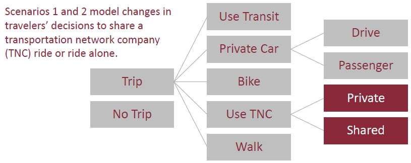
Figure 14. Graphic. Explanation of modes and decisions affected by scenarios 1 and 2.
(Source: Federal Highway Administration)
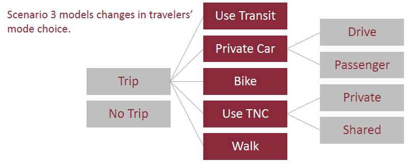
Figure 15. Graphic. Explanation of modes and decisions affected by scenario 3.
(Source: Federal Highway Administration)
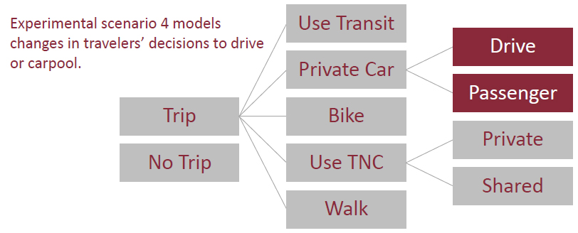
Figure 16. Graphic. Explanation of modes and decisions affected by experimental scenario 4.
(Source: Federal Highway Administration)
The analytic model presented in the following section is able to estimate the effects of these scenarios on particular market segments. The analytic model can also show how policy impacts would likely differ by city based on considerations such as average trip distances.
The scenario analysis results presented in the following section are built upon an analytic model constructed in R and available at Intelligent Transportation Systems (ITS) CodeHub, U.S. Department of Transportation's (USDOT) portal for open-source ITS code. Readers can download the code from the ITS CodeHub9 and run the analytic model to further explore the findings of the research in this report. The model allows the user to conduct their own tests, such as of a preferred policy scenario at a particular price point, for the fifteen cities included in the model. The model allows the user to explore the findings of the research described in chapters 2 and 3 as applied to the scenarios defined above.
The model can be used to explore changes in mode choice that might be observed if the relative time and price of various transportation modes were to change. The model allows testing of the scenarios that were developed from the research that the Federal Highway Administration (FHWA) explored on price and time but does not analyze all the potential policies that could impact modal choice. Despite the lack of perfect information on interactions between scenarios, the model offers the user the ability to test more than one scenario concurrently. For example, the user may apply scenarios for changes affecting personal cars and ridehailing simultaneously.
The "Scenarios" tab allows the user to apply different levels and combinations of the scenarios (see figure 17). A slider bar is provided for each of the scenarios. The maximum value of each slider bar is determined according to the limits of the research into the effects of each scenario (e.g., price differences between private and shared TNC rides of greater than $4 per mile were not queried and so the analytic model was designed to not allow inputs outside of this range).
The "Segments" tab allows the user to narrow the scenario analysis by geography, population segment, and time of day (see figure 17). The "Geography" menu allows the user to select between the 15 study cities analyzed in Chapter 1 or to select "All Study Cities." The "Population Segment" menu allows the user to select between the segments for which models were re-estimated, as described in chapter 1 (i.e., annual income, relative gross office and industrial employment density for the market at the trip origin and destination, regional centrality index by transit at the trip origin and destination, and trips to/from airports or other intermodal hubs). Finally, the user can also toggle between peak period trips (i.e., trips beginning between 8:00 and 9:59 a.m. or 4:00 p.m. and 6:59 p.m.) or all trips. All segments affect the number of trips and amount of VMT included in the model outputs, with each additional segmentation reducing the number of trips affected. Population segment sizes are calculated using data from NHTS 2016 and from the TNC survey.
The "Customize Initial Mode Shares" tab allows the user to input customized initial mode shares (by person trip) for analysis (see figure 17). By default, mode shares are derived from National Household Travel Survey 2016 data. However, the user may override this starting point with more current or localized information. Any mode share may be entered as long as the sum of the shares is 100 percent. Throughout the analytic model, "mode share" refers to person trips.
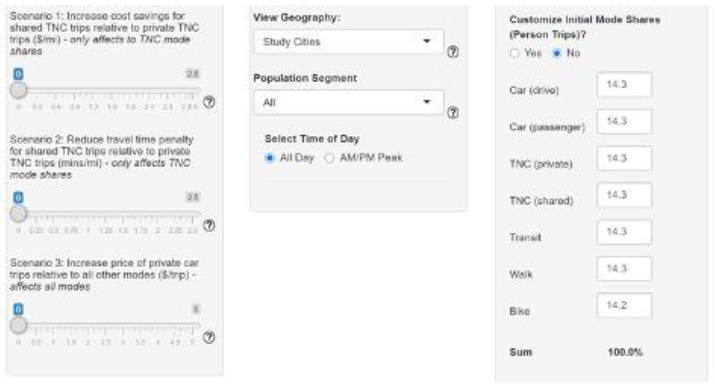
Figure 17. Image. Screenshots, from left to right: "Scenarios" sidebar tab, "Segments" sidebar tab, and "Customize Initial Mode Shares" sidebar tab.
(Source: Federal Highway Administration)
The user can override these defaults using the slider bars. The question mark boxes provide citations or explanations for each of the assumptions. For convenience, these explanations are listed below:
Trips Affected by Car Pricing Policies: This value affects the impact of scenario 3, which impacts private car trips. This value can be used to tailor the scenario definition to be specific to the type of policy instrument applied. For example, a 100 percent value here means that the price difference would affect all vehicle trips for the selected segment. A lower share would be appropriate for a smaller cordon, or parking surcharge-based policy instrument (as not all parking is controlled). This assumption can also represent policy instrument leakage, since some number of vehicles may find their way around parking or cordon charges according to specific limitations or exemptions of any ultimate policy. In consideration of this effect, the default value is 70 percent.
Penetration of Carpooling Incentive Apps: This value represents the share of travelers that would opt in to using a carpooling app, which supports the use of reward incentives. The default value is 25 percent.
Vehicle Occupancy for Carpool Trips (before applying scenarios): This value represents the occupancy of carpool trips prior to the application of scenario 3 and/or Experimental scenario 4, which would be expected to impact the occupancy of carpool trips. The default starting occupancy of carpool trips is 2.05 people per vehicle.
Vehicle Occupancy for Carpool Trips (after applying scenarios): This value represents the new occupancy after applications of scenario 3 and/or experimental scenario 4. If, for example, there is a conversion of 2-person carpools to 3-person carpools as the result of the scenarios, then this value should be expected to increase. If the user assumes that all new carpool trips are created from former SOV trips, then this value can be set equal to vehicle occupancy for carpool trips before applying the scenarios. The default starting occupancy of carpool trips is 2.05 people per vehicle.
Shared TNC Overlap Rate: This value captures the percent of trips in which a user who opts in to sharing is matched with another rider (defaulted to 50 percent) and the percent of their trip where two parties are in vehicle (defaulted to 70 percent). Multiplying these two values together results in a starting value of 35 percent. It is needed to translate TNC mode share and trip distance into VMT. This value is within the range of plausible values suggested by Schaller.10 Another paper from Tachet et al. developed a formula predicting a related quantity they call shareability: the fraction of individual trips that can be shared within a tolerable threshold of delay.11 Using data on taxi trips in several cities in the United States and abroad, the authors computed a universal shareability curve based on a few basic characteristics, including trips per hour per area, providing evidence that shareability (a proxy for the shared TNC overlap rate) should increase along with spatiotemporal trip density. For that reason, an overlap rate greater than 35 percent may be feasible at greater levels of opt-in to shared TNC rides and also in cities with relatively high densities.
TNC Non-Passenger Miles: This value represents the share of TNC VMT without a passenger (i.e., cruising and deadheading). It is needed to translate TNC mode share and trip distance into VMT. The starting value of 42 percent is drawn from Balding et al.12
Pool Circuity: This value represents the additional distance that a shared TNC trip travels to accommodate matched parties when compared with a private TNC trip's more direct route. It is needed to translate TNC mode share and trip distance into VMT. The starting value is assumed to be 10 percent.
Carpool Circuity: This value represents the additional distance a carpool driver would travel to pick up his/her passenger relative to driving alone directly to his/her destination. It is needed to translate carpool mode share into VMT. The starting value is assumed to be 10 percent.
The analytic model processes the inputs described above (and shown in figure 18) and produces two primary outputs in its main panel: a table of values and a histogram of mode shares before and after the application of the scenario(s) being tested. (See figure 19.) The bars in the histogram represent the values presented in the "Initial Share" and "New Share" columns of the table. The figure also summarizes the change in VMT associated with the changes in mode share. Note that VMT is presented as "N/A" for several modes: passenger in private car, transit, walk, and bike. VMT associated with private car passenger trips is combined with private car VMT in the top row of the output table. Walking and biking require no motor vehicle travel. Transit VMT is omitted from this analysis because VMT per passenger mile traveled is so low in high-occupancy transit so as to be considered negligible, and transit VMT is unlikely to change significantly with changes in transit vehicle occupancy.
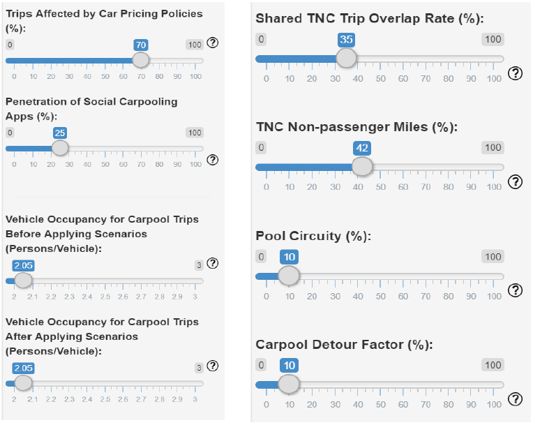
Figure 18. Image. Screenshot of slider bars features in "Assumptions" sidebar tab.
(Source: Federal Highway Administration)
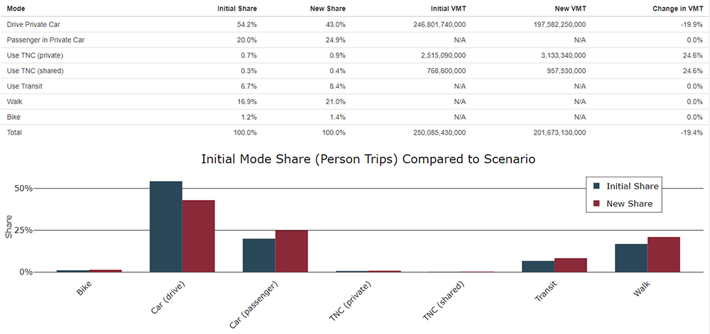
Figure 19. Graph. Sample output of analytic model for illustrative purposes.
(Source: Federal Highway Administration)
This analytic model is intended to assess the mode choice implications of relative price and travel time differences between single-occupancy/single-party and carpool/shared trips. These differences sometimes result from public policy but could also stem from market dynamics or corporate pricing policy. The analytic model is agnostic as to the source of these differences.
As noted in chapter 2, the results of the TNC survey research built into the analytic model are limited by the trip alternative questions asked in the survey. That is, the study did not produce the data to evaluate the effects of price and time differences that exceed those presented in Table 3 (i.e., maximum shared TNC discount of 75 percent). It is not possible, for example, for the analytic model to assess the effects of free shared TNC trips on the rate at which people choose to use shared TNCs. For that reason, the maximum allowable input values for scenarios 1 and 2 are capped at $2.80/mile and 2.5 minutes/mile respectively. These limits are calculated by multiplying the highest level of price difference (75 percent) or travel time difference (approximately 65 percent) included in the survey by the observed average price per mile ($3.30) or travel duration per mile (3.9 minutes).
Except for scenario 3, interactions across all modes are not considered. As shown in figure 16, the first and second scenarios reallocate trips between TNCs (private and shared) and as shown in figure 15, the third scenario reallocates only between private vehicles (drive alone or carpool). These reallocation patterns should still provide interesting insights and may not be too far from accurate, because (1) travelers typically seem to make decisions between personal cars, for-hire vehicles, transit, and active transportation before making decisions about shared versus private personal cars and for-hire vehicles; and (2) the relative prices of the first-order choices remain the same regardless of changes within the categories.
In scenario 3, "Drive Private Car" trips are reallocated to other modes according to initial mode share. For this scenario (and the others), the research does not consider either induced demand or, conversely, that some people may choose not to travel if mode characteristics change.
Finally, the analytic model is built on a number of assumptions that are explained in pop-up question mark text in the "Assumptions" tab and described above. These assumptions may be updated within the analytic model if better, more current, and/or more localized information becomes available.
The following section uses the analytic model described above to assess the VMT impact of various scenario applications in multiple cities and across multiple population segments. Figure 20 presents a high-level summary of the effect of various levels for three scenarios, plus a combination of scenarios 1 and 2.
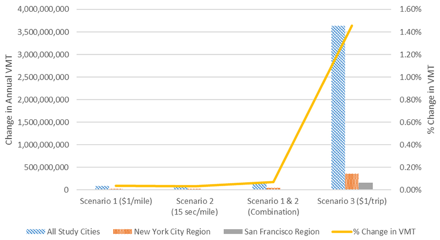
Figure 20. Graph. Effect of scenarios on vehicle miles traveled (total change and percent change).
(Source: Federal Highway Administration)
Key findings displayed in figure 20 include:
The following sections present greater detail on the effect of each of the three scenarios.
Table 19 tests the effect of scenario 1 on VMT. The analytic model allows the user to test the scenario at any price level from $0.05 to $2.80 per mile. The results in Table 19 present the effect of a $1/mile increase in the price difference between private and shared TNCs—a meaningful, but realistic increase in the difference in price between these two modes. The effect of a higher or lower price difference on VMT would scale linearly to the size of the price difference and effect presented here. The table presents the results for all trips (on the left) and for trips starting in dense office districts (on the right). This segment was chosen because trips in that segment were shown to be more sensitive to this price difference (as described in figure 5). Table 19 also presents three geographies. The table only presents TNC VMT (and total VMT by all modes) because scenario 1 does not affect private vehicle, transit, walk, or bicycle modes.
As expected, table 19 shows that the effect of scenario 1 on VMT is more than twice as great for trips starting in dense office districts (i.e., annual VMT savings of 0.09 percent compared to 0.04 percent for all trips). Due to the higher initial share of TNC trips, the effect of scenario 1 on VMT is proportionally higher in New York City and San Francisco than for the study cities taken as a whole (i.e., VMT reductions of 0.06 to 0.07 percent compared to 0.04 percent). Considering all trips in all study cities, a $1 additional price difference (per mile) between private and shared TNCs would reduce VMT by roughly 88 million miles per year by reducing private TNC VMT by 12.3 percent and substituting shared TNCs for that travel.
Table 20 shows the effect of scenario 2 on VMT. The analytic model allows the user to test the scenario at any level up to 2.5 minutes per mile. The results in table 20 present the effect of a 15 seconds/mile travel time difference reduction (between private and shared TNCs), a VMT impact roughly equivalent to the $1/mile impact shown in table 19. As with scenario 1, the effect of a higher or lower travel time difference on VMT would scale linearly to the size of the difference tested. The table presents the results for all trips (on the left) and for trips ending in dense office districts (on the right). This segment was chosen because trips in that segment were shown to be more sensitive to this time difference (as described in figure 7). The table only presents TNC VMT (and total VMT by all modes) because scenario 2 does not affect private vehicle, transit, walk, or bicycle modes.
As expected, table 20 shows that the effect of scenario 2 on VMT is greater for trips ending in dense office districts (i.e., annual VMT savings of 0.05 percent compared to 0.03 percent for all trips). Due to the higher initial share of TNC trips, the effect of scenario 2 on VMT is proportionally higher in New York City and San Francisco than for the study cities taken as a whole (i.e., VMT reductions of 0.06 to 0.07 percent compared to 0.03 percent). Considering all trips in all study cities, a 15 seconds per mile travel time difference reduction between private and shared TNCs would reduce VMT by roughly 85 million miles per year by reducing private TNC miles by 11.9 percent and substituting shared TNC travel for that difference.
| Geo-graphy | All Trips | Trips Starting in Dense Office Districts | |||||||||
|---|---|---|---|---|---|---|---|---|---|---|---|
| Use TNC Mode | Initial Share (%) | New Share (%) | Initial Vehicle Miles Traveled (VMT) | New VMT | Change in VMT (%) | Initial Share (%) | New Share (%) | Initial VMT | New VMT | Change in VMT (%) | |
| All Study Cities | Private | 0.7 | 0.6 | 2,515,090,000 | 2,205,760,000 | -12.30 | 0.7 | 0.5 | 418,770,000 | 285,120,000 | -31.90 |
| Shared | 0.3 | 0.4 | 768,600,000 | 989,770,000 | 28.80 | 0.3 | 0.6 | 127,970,000 | 223,540,000 | 74.70 | |
| Total | 1.0 | 1.0 | 3,283,690,000 | 3,195,530,000 | -2.7 | 1.0 | 1.1 | 546,740,000 | 508,660,000 | -6.96 | |
| Total all modes | 100.0 | 100.0 | 250,085,430,000 | 249,997,270,000 | -0.04 | 100.0 | 100.0 | 41,640,200,000 | 41,602,110,000 | -0.09 | |
| New York City Region | Private | 1.2 | 1.1 | 636,050,000 | 550,980,000 | -13.40 | 1.2 | 0.8 | 105,910,000 | 69,150,000 | -34.70 |
| Shared | 0.7 | 0.8 | 251,180,000 | 312,010,000 | 24.20 | 0.7 | 1.1 | 41,820,000 | 68,100,000 | 62.80 | |
| Total | 1.9 | 1.9 | 887,230,000 | 862,990,000 | -2.73 | 1.9 | 1.9 | 147,730,000 | 137,250,000 | -7.09 | |
| Total all modes | 100.0 | 100.0 | 33,012,550,000 | 32,988,310,000 | -0.07 | 100.0 | 100.0 | 5,496,720,000 | 5,486,240,000 | -0.19 | |
| San Francisco Region | Private | 1.0 | 0.9 | 197,710,000 | 171,030,000 | -13.50 | 1.0 | 0.7 | 32,920,000 | 21,390,000 | -35.00 |
| Shared | 0.6 | 0.7 | 80,544,000 | 99,070,000 | 23.80 | 0.6 | 0.9 | 13,320,000 | 21,560,000 | 61.90 | |
| Total | 1.6 | 1.6 | 278,254,000 | 270,100,000 | -2.93 | 1.6 | 1.6 | 46,240,000 | 42,950,000 | -7.12 | |
| Total all modes | 100.0 | 100.0 | 11,728,310,000 | 11,720,710,000 | -0.06 | 100.0 | 100.0 | 1,952,810,000 | 1,949,530,000 | -0.17 | |
Key: TNC: Transportation Network Company
| Geo-graphy | All Trips | Trips Ending in Dense Office Districts | |||||||||
|---|---|---|---|---|---|---|---|---|---|---|---|
| Use TNC Mode | Initial Share (%) | New Share (%) | Initial Vehicle Miles Traveled (VMT) | New VMT | Change in VMT (%) | Initial Share (%) | New Share (%) | Initial VMT | New VMT | Change in VMT (%) | |
| All Study Cities | Private | 0.7 | 0.7 | 2,515,090,000 | 2,216,610,000 | -11.90 | 0.7 | 0.6 | 681,120,000 | 572,670,000 | -15.90 |
| Shared | 0.3 | 0.4 | 768,600,000 | 982,020,000 | 27.80 | 0.3 | 0.4 | 208,150,000 | 285,690,000 | 37.30 | |
| Total | 1.0 | 1.1 | 3,283,690,000 | 3,198,630,000 | -2.6 | 1.0 | 1.0 | 889,270,000 | 858,360,000 | -3.48 | |
| Total all modes | 100.0 | 100.0 | 250,085,430,000 | 250,000,360,000 | -0.03 | 100.0 | 100.0 | 67,726,220,000 | 67,695,310,000 | -0.05 | |
| New York City Region | Private | 1.2 | 1.1 | 636,050,000 | 553,960,000 | -12.90 | 1.2 | 1.0 | 172,250,000 | 142,420,000 | -17.30 |
| Shared | 0.7 | 0.8 | 251,180,000 | 309,880,000 | 23.40 | 0.7 | 0.9 | 68,020,000 | 89,350,000 | 31.40 | |
| Total | 1.9 | 1.9 | 887,230,000 | 863,840,000 | -2.64 | 1.9 | 1.9 | 240,270,000 | 231,770,000 | -3.54 | |
| Total all modes | 100.0 | 100.0 | 33,012,550,000 | 32,989,160,000 | -0.07 | 100.0 | 100.0 | 8,940,210,000 | 8,931,710,000 | -0.10 | |
| San Francisco Region | Private | 1.0 | 0.9 | 197,710,000 | 171,970,000 | -13.00 | 1.0 | 0.8 | 53,540,000 | 44,190,000 | -17.50 |
| Shared | 0.6 | 0.7 | 80,544,000 | 98,400,000 | 23.00 | 0.6 | 0.8 | 21,660,000 | 28,350,000 | 30.90 | |
| Total | 1.6 | 1.6 | 278,254,000 | 270,370,000 | -2.83 | 1.6 | 1.6 | 75,200,000 | 72,540,000 | -3.54 | |
| Total all modes | 100.0 | 100.0 | 11,728,310,000 | 11,720,980,000 | -0.06 | 100.0 | 100.0 | 3,176,170,000 | 3,173,510,000 | -0.08 | |
Key: TNC: Transportation Network Company
Table 21 presents the impacts on VMT, at the level of $1/mile and 15 seconds per mile, respectively. These effects were chosen to represent a realistic, multifaceted approach to reduction of TNC VMT. As before, the table presents the results for all trips (on the left) and for trips ending in dense office districts (on the right), and for three geographies.
Because it is assumed in this study that the effects of travel time and price differences are linear for the values tested in the study, combining scenarios 1 and 2 simply adds the effect of the two scenarios together. As expected, table 21 shows a VMT effect greater than either scenario 1 or scenario 2 alone, for all cities and for any segment. Considering all trips in all study cities, a $1 additional price difference between private and shared TNCs combined with a 15 second/mile travel time advantage would reduce VMT by roughly 173 million miles per year.
| Geo-graphy | All Trips | Trips Ending in Dense Office Districts | |||||||||
|---|---|---|---|---|---|---|---|---|---|---|---|
| Use TNC Mode | Initial Share | New Share | Initial Vehicle Miles Traveled (VMT) | New VMT | Change in VMT | Initial Share | New Share | Initial VMT | New VMT | Change in VMT | |
| All Study Cities | Private | 0.7 | 0.6 | 2,515,090,000 | 1,907,280,000 | -24.20 | 0.7 | 0.5 | 681,120,000 | 486,040,000 | -28.60 |
| Shared | 0.3 | 0.5 | 768,600,000 | 1,203,190,000 | 56.50 | 0.3 | 0.5 | 208,150,000 | 347,630,000 | 67.00 | |
| Total | 1.0 | 1.1 | 3,283,690,000 | 3,110,470,000 | -5.3 | 1.0 | 1.0 | 889,270,000 | 833,670,000 | -6.25 | |
| Total all modes | 100.0 | 100.0 | 250,085,430,000 | 249,912,200,000 | -0.07 | 100.0 | 100.0 | 67,726,220,000 | 67,670,620,000 | -0.08 | |
| New York City Region | Private | 1.2 | 0.9 | 636,050,000 | 468,890,000 | -26.30 | 1.2 | 0.8 | 172,250,000 | 118,600,000 | -31.10 |
| Shared | 0.7 | 1.0 | 251,180,000 | 370,700,000 | 47.60 | 0.7 | 1.1 | 68,020,000 | 106,380,000 | 56.40 | |
| Total | 1.9 | 1.9 | 887,230,000 | 839,590,000 | -5.37 | 1.9 | 1.9 | 240,270,000 | 224,980,000 | -6.36 | |
| Total all modes | 100.0 | 100.0 | 33,012,550,000 | 32,964,910,000 | -0.14 | 100.0 | 100.0 | 8,940,210,000 | 8,924,920,000 | -0.17 | |
| San Francisco Region | Private | 1.0 | 0.8 | 197,710,000 | 145,290,000 | -26.50 | 1.0 | 0.7 | 53,540,000 | 36,720,000 | -31.40 |
| Shared | 0.6 | 0.9 | 80,544,000 | 117,470,000 | 46.80 | 0.6 | 0.9 | 21,660,000 | 33,690,000 | 55.50 | |
| Total | 1.6 | 1.7 | 278,254,000 | 262,760,000 | -5.57 | 1.6 | 1.6 | 75,200,000 | 70,410,000 | -6.37 | |
| Total all modes | 100.0 | 100.0 | 11,728,310,000 | 11,713,380,000 | -0.13 | 100.0 | 100.0 | 3,176,170,000 | 3,171,380,000 | -0.15 | |
Key: TNC: Transportation Network Company
Table 22 shows the effect of scenario 3 on VMT, at a level of $1/private car trip. The effect on VMT presented here (a 1.45 percent reduction in VMT across all study city regions) is greater than the effect observed in either of the TNC scenarios (scenarios 1 and 2), where VMT reductions ranged from 0.03 percent to 0.17 percent. Considering all trips in all study city regions, a $1/trip relative price increase for "Drive Private Car" would reduce VMT by roughly 3.6 billion miles per year. This effect is greater than the VMT reductions of scenarios 1 and 2 because scenario 3 affects many more trips; while driving alone accounts for 54.2 percent of trips in the study city regions, private TNC trips account for less than 1 percent in the study city regions.
Unlike the previous tables in this section, this table presents the results only for all trips as the scenario effect studied is not shown to vary between population segments. That is, although the amount of VMT within a segment does differ (i.e., there are more total trips than trips to the airport), the analytic model assumes that a $1/trip price increase for private car travel would have a proportional effect on any segment.
Table 22 presents three geographies. Unlike the other tables in this section, this table presents VMT for all modes because scenario 3 shifts trips from private vehicles to other modes: TNC, transit, walk, and bicycle.
| Geography | Mode | Initial Share (%) | New Share (%) | Initial Vehicle Miles Traveled (VMT) | New VMT | Change in VMT (%) |
|---|---|---|---|---|---|---|
| All Study Cities | Drive private car | 54.2 | 53.4 | 246,801,740,000 | 243,103,410,000 | -1.50 |
| Passenger in private car | 20.0 | 20.4 | N/A | N/A | 0.00 | |
| Use transportation network company (TNC) (private) | 0.7 | 0.8 | 2,515,090,000 | 2,561,550,000 | 1.85 | |
| Use TNC (shared) | 0.3 | 0.3 | 768,600,000 | 782,790,000 | 1.85 | |
| Use TNC (total) | 1.0 | 1.1 | 3,283,690,000 | 3,344,340,000 | 1.85 | |
| Use transit | 6.7 | 6.9 | N/A | N/A | 0.00 | |
| Walk | 16.9 | 17.2 | N/A | N/A | 0.00 | |
| Bike | 1.2 | 1.2 | N/A | N/A | 0.00 | |
| Total | 100.0 | 100.0 | 250,085,430,000 | 246,447,760,000 | -1.45 | |
| New York City Region | Drive private car | 42.1 | 41.6 | 32,125,320,000 | 31,765,270,000 | -1.12 |
| Passenger in private car | 16.4 | 16.5 | N/A | N/A | 0.00 | |
| Use TNC (private) | 1.2 | 1.2 | 636,050,000 | 641,400,000 | 0.84 | |
| Use TNC (shared) | 0.7 | 0.7 | 251,180,000 | 253,290,000 | 0.84 | |
| Use TNC (total) | 1.9 | 1.9 | 887,230,000 | 894,690,000 | 0.84 | |
| Use transit | 13.0 | 13.1 | N/A | N/A | 0.00 | |
| Walk | 25.5 | 25.7 | N/A | N/A | 0.00 | |
| Bike | 1.2 | 1.2 | N/A | N/A | 0.00 | |
| Total | 100.0 | 100.0 | 33,012,550,000 | 32,659,960,000 | -1.07 | |
| San Francisco Region | Drive private car | 48.6 | 48.5 | 11,450,610,000 | 11,287,400,000 | -1.43 |
| Passenger in private car | 22.0 | 22.3 | N/A | N/A | 0.00 | |
| Use TNC (private) | 1.0 | 1.0 | 197,710,000 | 200,500,000 | 1.41 | |
| Use TNC (shared) | 0.6 | 0.6 | 80,000,000 | 81,120,000 | 1.40 | |
| Use TNC (total) | 1.6 | 1.6 | 277,710,000 | 281,620,000 | 1.41 | |
| Use transit | 7.1 | 7.2 | N/A | N/A | 0.00 | |
| Walk | 18.8 | 19.1 | N/A | N/A | 0.00 | |
| Bike | 1.9 | 1.9 | N/A | N/A | 0.00 | |
| Total | 100.0 | 100.0 | 11,728,310,000 | 11,569,020,000 | -1.36 |
1 A cordon could delineate an airport area, a downtown, an important highway link, or any other zone or facility. Cordon-based policies could be applied to some or all vehicles entering, all trips terminating (for-hire or privately-owned and parked), or only vehicles garaged in a zone. [ Return to Note 1 ]
2 This could be implemented as a percentage of a TNC's time per hour that could be allocated to private trips in order to avoid restricting growth of upstart TNCs or competition between TNCs to secure all the allowable private trips within an hour. [ Return to Note 2 ]
3 Shoup et al (2005) [ Return to Note 3 ]
4 Concas, S. and Nayak, N. (2012). "A Meta-analysis of Parking Pricing Elasticity." [ Return to Note 4 ]
5 Farber, M. and Weld, E. (2013). Econometric Analysis of Public Parking Price Elasticity in Eugene, Oregon. [ Return to Note 5 ]
6 Litman, T. (2013). Understanding Transport Demands and Elasticities: How Prices and Other Factors Affect Travel Behavior. [ Return to Note 6 ]
7 Hymel, K.M., Small, K.A., and Van Dender, K. (2010). "Induced Demand and Rebound Effects in Road Transport." [ Return to Note 7 ]
8 Concas, S. and Nayak, N. (2012). [ Return to Note 8 ]
9 Direct link to the project repository: https://doi.org/10.21949/1520429 [ Return to Note 9 ]
10 Schaller, B. (2018). [ Return to Note 10 ]
11 Tachet, R., Sagarra, O., Santi, P., Resta, G., Szell, M., Strogatz, S.H., and Ratti, C. (2017). "Scaling Law of Urban Ride Sharing." [ Return to Note 11 ]
12 Balding, M., Whinery, T., Leshner, E., and Womeldorff, E. (2019). [ Return to Note 12 ]
|
United States Department of Transportation - Federal Highway Administration |
||