Freight Mobility Trends Report 2019APPENDIX A: DATA, MEASURES, AND METHODOLOGYDataThe Federal Highway Administration’s (FHWA) Freight Mobility Trends (FMT) relies on the National Performance Management Research Data Set (NPMRDS) and Highway Performance Monitoring System (HPMS) data sets, described as follows:
Data ProcessingThe basic spatial unit of analysis is the TMC. This is a relatively short directional roadway segment that is defined by a consortium of commercial traffic information providers. The travel time data were averaged to 15-minute time bins. Then, the FMT indices were calculated for each TMC on the National Highway System (NHS) from the raw NPMRDS data. Further, TMC measures were placed on the segments, and length or volume was used to weight the index measures to obtain aggregate measures. SegmentationSegmentation included auto-segmenting the NHS into approximately 3- to 9-mile sections in urban locations (those that contain at least part of an urban area) and 5- to 10-mile sections in rural areas. This provides a better way to visualize problem areas because many of the TMC links are so short they will not show up in a zoomed-out map when analyzed. The longer segment lengths are also more representative of typical freight project limits, rather than the occasional, short TMC lengths that show up (e.g., 0.1 miles). This processing method allows aggregation and the ability to report freight congestion statistics at various geographies, because all calculations are still performed at the TMC level but aggregated to different geographies based on weighting (described later). Reference SpeedThe reference speed (sometimes called off-peak, uncongested, or baseline speed) used for the FMT is based on a calculated free-flow (reference) speed using the NPMRDS travel times. This approach was used rather than using the posted speed limit, because speed limits for all vehicles do not always reflect typical free-flow speeds for large trucks. Reference speed has proven effective because it is a direct measurement of traffic conditions and varies when geometric changes are on the roadway (e.g., added lanes). The reference speed calculation is similar to the method currently used in FHWA’s Urban Congestion Report for the Planning Time Index (PTI) and Travel Time Index (TTI).3 For the FMT, only truck data are used for the reference speed calculation. The FMT includes an index that is similar to the Truck Travel Time Reliability (TTTR) measures States are required to report under 23 CFR 490.607, but the FMT is slightly different. This index, the Truck Reliability Index (TRI), similarly uses the 95th percentile travel time compared to the 50th percentile travel time instead of the free-flow reference speed used by the other indicators. Measure WeightingWeighting is reflected in the index calculations. All mobility indices (TTI, PTI, and Buffer Index (BI)) are weighted by Truck Vehicle Miles Traveled (TVMT) to allow for aggregating up to section, area, State, and national values. Definitions and CalculationsThe suite of indicators includes the following:
DelayDelay represents the amount of extra time spent traveling due to congestion. The FMT uses two measures of delay: total delay and delay per mile. Total DelayTotal delay is calculated by adding up all the delay (at 15-minute intervals for this example) for each TMC across the area being analyzed for a specific time period (year, quarter, or month) and is defined in figure 61. 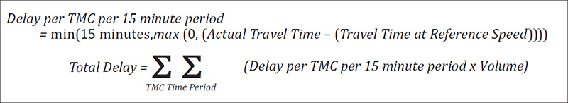
Figure 61. Formula. Total delay calculation. When calculating delay, rather than just using reference speed for missing values (where no delay is accumulated), missing travel times are estimated from historical observations. The observations come from the last 12 months, starting with the average week of the year, which consists of 96 15 minute periods for each of the seven days of the week (96 × 7). If there is not a historical value in the 96 × 7 average, an hourly average for each day of the week will be used (24 × 7). This will continue to 96 × 2 (96 15-minute periods by weekday and weekend) and 24 × 2 (24 hourly periods by weekday and weekend) before using just the weekday or weekend average and finally just taking the yearly average. In summary, the imputed travel times for missing values were assigned in the following trickle-down manner, where each subsequent step is only taken if the data from the current step are not available:
Delay per Mile (for Sections)Delay per mile is the total delay for a section of roadway divided by the section length. This is calculated for the entire NHS for the FMT. MobilityThe following defines and illustrates calculations for the recommended mobility indices. Travel Time IndexThe TTI compares peak-period travel time to free-flow travel time. The TTI includes both recurring and incident conditions. The ratio has components of time divided by time. Therefore, it has no units. This unit-less feature allows the index to be used to compare trips of different lengths to estimate the travel time in excess of that experienced in reference travel time (free-flow travel time) conditions. The TTI is the ratio of the peak-period travel time to the reference travel time (free-flow travel time). This measure is computed for the AM peak period (6 a.m. to 9 a.m.) and PM peak period (4 p.m. to 7 p.m.) on weekdays. The TTI is calculated as in figure 62. 
Figure 62. Formula. Travel time index equation. To calculate the average TTI across urban areas, road sections and time periods are weighted by vehicle miles traveled using volume estimates derived from FHWA’s HPMS. ReliabilityPlanning Time IndexThe PTI is the ratio of the 95th percentile travel time to the reference travel time (free-flow travel time). The measure is computed during the AM and PM peak periods as defined in the TTI. PTI is calculated as figure 63. 
Figure 63. Formula. Planning time index equation. The PTI is based on the concept that travelers want to be on time for an important trip 19 out of 20 times. For example, a PTI value To calculate the average PTI across urban areas, road sections and time periods are weighted by TVMT using volume estimates derived from FHWA’s HPMS. Buffer IndexThe BI represents the extra time (or time cushion) that travelers must add to their average travel time when planning trips to ensure on-time arrival. For example, a BI of 40 percent means that for a trip that usually takes 20 minutes, a traveler should budget an additional eight minutes (20 minutes × 0.40). The eight extra minutes is called the buffer time. Therefore, the traveler should allow 28 minutes for the trip to ensure on-time arrival 95 percent of the time. The BI is calculated as in figure 64. 
Figure 64. Formula. Buffer index equation. Truck Reliability IndexThe TRI calculation is similar to the MAP 21 performance measure for TTTR. The TRI indicator uses the same five time periods as the TTTR performance measure:
The TRI is calculated as in figure 65. 
Figure 65. Formula. Truck reliability index equation. The TRI was generated in accordance with 23 CFR § 490.613 by multiplying the largest ratio of the five time periods by its length and then dividing the sum of all length-weighted segments by the total length (figure 66).4 
Figure 66. Formula. Truck reliability index. The TRI in the FMT cannot be used to report the official MAP-21 TTTR performance measure. The FMT tool uses different roadway segmentation with TMCs combined to longer corridors for analysis. Because of this, the TRI generated by the FMT tool will not match the NPMRDS-generated TTTR performance measure. The TRI in the FMT is used to analyze reliability trends and cannot be used to report the official MAP-21 TTTR performance measure. Bottleneck Identification CriteriaThis report also includes information on national bottlenecks. A ranking of roadway sections is based on the FMT calculations for delay per mile. Though it is also possible to rank bottlenecks by any number of the measures and break them out by rural and urban, FHWA uses delay per mile as the primary measure because it includes the full extent of the truck congestion problem for all days throughout the year. This is the primary measure and method in current bottleneck ranking products such as the Texas 100 Most Congested Roadways.5 Delay per mile conveys the magnitude of the problem, captures a 365 day/24-hour/7-day view of the problem, and is normalized by length so that varying-length roads can be compared.6 Corridor CalculationsFor analysis of freight corridors (which are defined in the “Locations” section of this appendix), the indicators require some context to the traditional calculations of these indices. For the TTI, there is a comparison of a peak time to a free-flow travel time. For the PTI, there is a comparison of the 95th percentile travel time to the free-flow travel time. Because the freight corridors extend for long distances, defining when peak and free flow occur along the entire corridor is challenging. Additionally, delay is difficult to calculate over a long trip where there are different volumes and free-flow speeds on different sections of the corridor. To show the corridor performance, travel time traces were computed for the length of the corridor, which is modeling vehicles over time and space that would travel the corridor. Then, a BI was computed from the distribution of the resulting data. LocationsThe FMT tool provides a suite of indicators across the entire NHS at a variety of location categories. The location categories include road types nationally, at the State level, and then in urban and rural areas. The categories also include border crossing, metropolitan, and intermodal locations. Having data and indices for the entire NHS provides the flexibility to see performance everywhere and focus on specific locations that may be driving freight performance. For example, if the national roll-up number changes, the user can look at the different spatial levels (zoom in or out) to see where freight mobility may be influencing the national number. The categories reflected in this report are as follows. National Roll-Up MeasuresNational roll-up measures are applied for the entire NHS in aggregate for each of the indicators described previously. All National Highway System RoadsIn addition to the national roll-up, national-level measures are available for the following functional classes:
Urban National Highway System RoadsUrban NHS indices are available by the following functional classes:
Rural National Highway System RoadsRural NHS indices are available by the following functional classes:
State National Highway System RoadsState NHS indices are available by the following functional classes:
Freight CorridorsFHWA selected 30 freight corridors that are key facilities for freight movement throughout the United States. Figure 67 shows these corridors. BottlenecksThe FMT dashboard and the underlying segmentation of the NHS network allow use of delay per mile to provide an industry-tested ranking of bottlenecks. For this report, the FMT dashboard provided an output of the top-40 national bottlenecks using delay per mile. BordersThere are 20 northern border crossings with Canada and 6 southern border crossings with Mexico, all of which are included in the FMT. The FMT assesses the actual crossing segments into and out of either Canada or Mexico, as well as roads in the surrounding area that feed the border crossing. Urban RegionsThe FMT includes indicators for major urban areas with a population of 50,000 or more throughout the United States. Metropolitan Planning Organization RegionsThe FMT includes indicators for Metropolitan Planning Organization (MPO) regions throughout the United States. 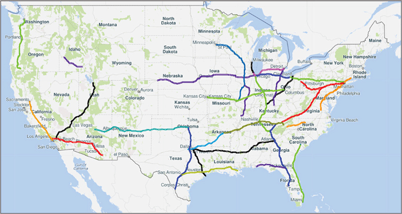
Source: FHWA National Highway Freight NetworkThe FMT assesses performance and includes indicators for the National Highway Freight Network (NHFN). Strategic Highway NetworkThe FMT assesses performance and includes indicators for the Strategic Highway Network (STRAHNET). PortsPorts reflected in this report were those aligned with the top ports based on the BTS port performance measures. BTS measures ports for tonnage, twenty-foot equivalent units (TEUs), and dry bulk. BTS uses this information to identify the top 25 locations for tonnage, container, and dry bulk.7 FHWA determined 25 port locations to monitor throughout the United States based on the top locations by selecting the 18 ports that are top ports for tonnage, TEUs, or dry bulk and then high vessel count data and tonnage from the Bureau of Transportation Statistics (BTS) to rank the remaining ports. The following port locations are included in this report:
AirportsFor the airport locations, the FMT includes the top 20 cargo-bearing airport locations as provided by BTS.8
Railroad TerminalsFor railroad intermodal locations, the FMT aligns with publicly available railroad dwell-time measures by including measures for NHS roads around key rail intermodal locations. Selected rail terminal locations include the following:
Appendix A References
|
|
United States Department of Transportation - Federal Highway Administration |
||