APPENDIX B. USING BAYESIAN INFERENCE TO UPDATE SCENARIO PROBABILITIES
Note: Unless accompanied by a citation to statute or regulations, the practices, methodologies, and specifications discussed below are not required under Federal law or regulations.
The joint probability distribution developed over the scenarios in step 5 of the approach could be updated using different techniques. As new information related to the scenarios become available (e.g., through field observations) and/or the analyst belief regarding the relative importance of various scenarios changes, the predefined joint probability distribution may need to be updated. One of the commonly used methods for updating probabilities is the Bayesian inference method. As a statistical inference method, Bayesian inference derives a posterior joint probability distribution by applying the Bayes’ theorem to the prior joint probability distribution of the scenarios. The following formula shows the Bayes’ rule.
Figure 95. Formula. Bayes’ rule.
Where Si is the ith scenario in the prior set of scenarios,  is the ith scenario in the posterior set of scenarios, P(Sk) refers to the prior probability of the kth scenario, and
  refers to the posterior probability of the kth scenario.
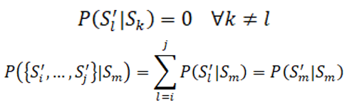
If there is complete information about each scenario in the prior and posterior stages, and if all the scenarios are mutually exclusive, the following relationships would be applicable.
Figure 96. Formula. Relationship between prior and posterior states of mutually exclusive scenarios.
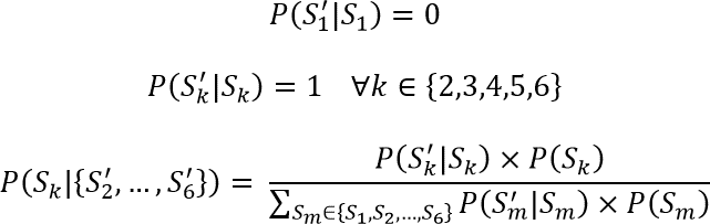
With these two assumptions the Bayes’ rule could be revised as follow:
Figure 97. Formula. Revised Bayes’ rule.
In this section, the following two types of examples for the probability updating process are provided using the first case study discussed in chapter 6.
The first case study was selected for these examples because of the mutual exclusiveness of the scenarios:
- Example 1 – One of the scenarios of the prior stage is removed in the posterior stage.
- Example 2 – The probabilities for a set of scenarios are updated in the posterior stage. The prior probabilities are listed in table 15.
Table 15. Prior probabilities for different demand scenarios.
Scenario |
Description |
Prior Probability |
1 |
Interarrival time increased by 20% for each path |
0.1 |
2 |
Interarrival process calibrated based on the I-290 traffic flow |
0.25 |
3 |
Interarrival time decreased by 20% for each path |
0.2 |
4 |
Interarrival time decreased by 40% for each path |
0.2 |
5 |
Interarrival time decreased by 60% for each path |
0.15 |
6 |
Interarrival time decreased by 80% for each path |
0.1 |
EXAMPLE 1
Let’s assume that over time it was realized that scenario 1 should be removed from the scenario set since it would not appear in future conditions of the system. Assuming that the ratio between the probabilities of any two scenarios (other than scenario 1) does not change in the prior and posterior stage, then the following relationships exist between the prior and posterior stages of the scenarios:
Figure 98. Equation. Relationship between prior and posterior probabilities in example 1.
The posterior probabilities calculated based on the above equations are shown in table 16.
Table 16. Prior and posterior probabilities for different demand scenarios in example 1.
Scenario |
Prior Probability |
Posterior Probability |
1 |
0.1 |
0 |
2 |
0.25 |
0.2778 |
3 |
0.2 |
0.2222 |
4 |
0.2 |
0.2222 |
5 |
0.15 |
0.1667 |
6 |
0.1 |
0.1111 |
EXAMPLE 2
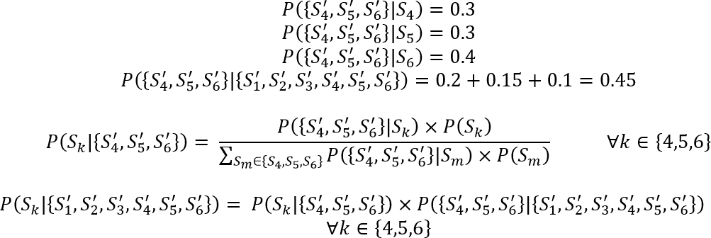
Now let’s assume that during the first three scenarios correspond to off-peak hour time periods and the last three scenarios correspond to peak hour time periods. If a set of observations during the peak hour shows that scenario 4, 5, and 6 occur 30 percent, 30 percent, and 40 percent of the times, respectively, then the probabilities of these three scenarios should be updated. In this situation, the off-peak period probabilities remain the same since no data s collected during the off-peak hours. The following relationships exist between the prior and posterior stages of the scenarios:
Figure 99. Equation. Relationship between prior and posterior probabilities in example 2.
The posterior probabilities calculated based on the above equations are shown in table 17.
Table 17. Prior and posterior probabilities for different demand scenarios in example 2.
Scenario |
Prior Probability |
Posterior Probability |
1 |
0.1 |
0.1 |
2 |
0.25 |
0.25 |
3 |
0.2 |
0.2 |
4 |
0.2 |
0.186 |
5 |
0.15 |
0.14 |
6 |
0.1 |
0.124 |