APPENDIX A. SUGGESTED NUMBER OF SCENARIOS AND NUMBER OF RUNS
Note: Unless accompanied by a citation to statute or regulations, the practices, methodologies, and specifications discussed below are not required under Federal law or regulations.
The number of simulations performed to achieve a desired level of accuracy in the results is an important element of studies that involve simulation. The time allocated to running the simulation tool and the available computational resources play a major role in determining this number. There are two numbers that should be determined for the framework proposed in this report: The number of scenarios to be analyzed, and the number of simulation runs for each scenario.
As discussed in chapter 7, if a joint probability distribution could be defined for the scenarios, the scenario-based analysis would be performed, otherwise, a robustness-based analysis is suggested. The type of analysis also influences the number of scenarios and simulations to be run. Under the scenario-based analysis, there is more knowledge about the scenarios and their probabilities.
Therefore, a limited number of scenarios could be analyzed but a higher number of simulation runs could be performed to derive more accurate results for each scenario. On the other hand, in the robustness-based analysis, due to lack of information about the possible set of the scenarios and no/ limited information about their associated probabilities, it is better to define a large number of scenarios. Analyzing a relatively comprehensive set of scenarios with a limited number of simulation runs provides an approximate output for each scenario but a better overall picture of the problem.
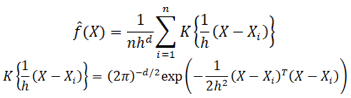
In most problems, it is not possible to test every possible scenario. As a result, the goal is to derive a distribution of the simulation tool outputs using a limited set of scenarios that closely matches the target distribution for the output. A smoothing method such as the multivariate kernel density estimation method could be utilized to approximate the target simulation output function by smoothing the curve developed by the outputs of the simulated scenarios. The following function represents the smoothed simulation output curve calculated as a function of a multivariate kernel density function such as the standard normal distribution:
Figure 91. Formula. Multivariate kernel density estimation formula.
Where  is the smoothed simulation output curve; X is the output of the simulation tool; Xi is the output of the simulation tool for the ith scenario; K is the kernel function; h is the smoothing parameter; d refers to the number of dimensions (number of varying parameters used to generate the scenarios); and n is the number of scenarios.
Figure 92 schematically represents how to smooth the simulation output by applying the kernel density estimation method. As shown in the figure, variations of two parameters were considered as the basis for developing different scenarios. Using these two dimensions, four distinct scenarios were generated. The three-dimensional diagram in the middle of the figure shows the outputs of the simulation tool for all the scenarios. By applying the kernel density estimation method, a smoothed curve such as the one shown on the right-hand side of the figure could be generated as an approximation of the target output over all feasible scenarios.
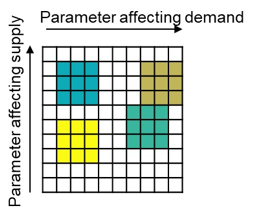
a) Scenario space.
This two-dimensional diagram schematically represents different scenarios based on the parameters affecting demand (x-axis) and the parameters affecting supply (y-axis). Four sample scenarios are depicted as rectangles. The scenarios are: 1) A scenario with low level of demand related parameters and low level of supply related parameters; 2) A scenario with low level of demand related parameters and high level of supply related parameters; 3) A scenario with high level of demand related parameters and medium level of supply related parameters; 4) A scenario with high level of demand related parameters and high level of supply related parameters.
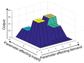
b) Simulation output.
This three-dimensional diagram schematically represents the simulation output (z-axis) for the different scenarios represented in the previous diagram based on the parameters affecting demand (x-axis) and the parameters affecting supply (y-axis). Four sample scenarios are depicted as boxes. The locations of the scenarios on the x- and y-axes are similar to the previous diagram. The z-axes for the scenarios are as follow: 1) Scenario 1: 80; 2) Scenario 2: 20; 3) Scenario 3: 40; 4) Scenario 4: 50.
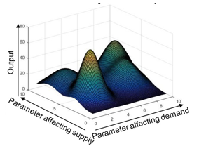
c) Smoothed simulation output
(applying kernel density estimation).
This three-dimensional diagram schematically represents the simulation output (z-axis) for the different scenarios represented in the previous diagram based on the parameters affecting demand (x-axis) and the parameters affecting supply (y-axis). The boxes in the previous graph are smoothed using a kernel density function to create an integrable surface.
Source: FHWA, 2019.
Figure 92. Illustration. Compound figure depicts the process of smoothing the simulation output using the multivariate kernel density estimation method.
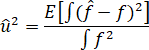
A measure that could be used to evaluate the quality of the approximated curve is the relative mean
integrated square error defined as follows:
Figure 93. Formula. Relative mean integrated square error.
The relative mean integrated square error (u hat square) equals (open parenthesis) the expected integral of the square of the difference between the smoothed simulation output curve (f hat) and the target function for the output (f) (close parenthesis) divided by the target function for the output (f).
Where  is the smoothed simulation output curve, and f is the target function for the output if all the feasible scenarios are simulated. If both curves and f are scaled so that the volume under the curve equals one, then the relative mean integrated square error varies between zero and one. Epanechnikov (1969) derived the required sample size (number of scenarios) to ensure that the relative mean square error at zero is less than a specified threshold, when estimating a standard multivariate normal density using a normal kernel and a smoothing parameter that minimizes the mean square error at zero (table 13). These values serve as a starting point to identify the minimum number of scenarios that should be simulated. Based on the general shape and the roughness of the target simulation output curve, the minimum required sample size could differ. Based on table 13, for example, if the simulation tool is used to analyze the effect of demand variation on a network and a relative mean integrated square error of less than 0.3 is acceptable, then it is suggested to define six scenarios with different demand levels. As another example, under the condition that a relative mean integrated square error of less than 0.2 is acceptable, if the effect of connected vehicles (CVs) and automated vehicles (AVs) on a network is studied, at least 21 scenarios should be generated. Therefore, five different market penetration rates for CVs and five for AVs could be determined. A total of 25 scenarios could be developed based on these two parameters.
Table 13. Suggested number of scenarios to simulate.
Minimum Number of Scenarios |
Relative Mean Integrated Square Error () |
0.1 |
0.2 |
0.3 |
0.4 |
0.5 |
d |
1 |
22 |
11 |
6 |
4 |
3 |
2 |
58 |
21 |
11 |
7 |
5 |
3 |
175 |
52 |
26 |
16 |
11 |
4 |
600 |
150 |
67 |
38 |
24 |
5 |
2220 |
470 |
190 |
98 |
59 |
Source: Epanechnikov 1969.
The number of simulation runs for each scenario is a function of:
- Variance in the simulation outputs (S2).
- Desired level of confidence (1−α).
- Desired range of confidence interval (CI1−α).
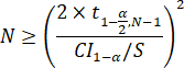
These three factors could vary for each scenario. As a result, the number of simulation runs could vary across the scenarios. Based on the above factors the following formula could be used to determine the minimum number of simulations per scenario.
Figure 94. Formula. Minimum number of simulation runs for each scenario.
The number of simulation run (N) is greater than or equal to (open parenthesis) 2 times the t-student critical value for a desired level of confidence (1 minus alpha) and a specified degree of freedom (N minus 1) (t subscript 1 minus alpha over 2 comma N minus 1) divided by (open parenthesis) the desired range of confidence interval (CI subscript 1 minus alpha) divided by the standard deviation in the simulation output (S) (close parenthesis) (close parenthesis) to the power of 2.
Table 14 provides suggested number of simulation runs calculated by the formula.
Table 14. Minimum number of simulation runs for each scenario.
Minimum Number of Simulation Runs |
Level of Confidence (1 – a) |
90% |
95% |
99% |
CI1-a/S |
0.5 |
64 |
84 |
131 |
1 |
18 |
23 |
36 |
1.5 |
10 |
12 |
19 |
2 |
6 |
8 |
12 |
2.5 |
5 |
6 |
9 |
3 |
4 |
5 |
8 |