Recurring Traffic Bottlenecks: A Primer
Focus on Low-Cost Operational Improvements (Fourth Edition)
Chapter 5. Analytical Identification and Assessment of Bottlenecks
Where Are the Bottlenecks and How Severe Are They?
Every highway facility has decision points such as on- and off-ramps, merge areas, weave areas, lane drops, tollbooth areas, and traffic signals; or design constraints such as curves, climbs, underpasses, and narrow or nonexistent shoulders. In many thousands of cases, these operational junctions and characteristics operate sufficiently and anonymously. However, when the design itself becomes the constricting factor in processing traffic demand, then an operationally influenced bottleneck can result.
The degree of congestion at a bottleneck location is related to its physical design and the volume overburden. Some operational junctions were constructed years ago using design standards now considered to be antiquated, while others were built to sufficiently high design standards but are simply overwhelmed by traffic demand. Bottlenecks, then, develop when both of these conditions exist; that is, an operational constraint that is acted upon by a traffic overburden. This is commonly "rush hour." Absent one or the other, the condition won't exist. The following sections provide some guidance on how to identify bottleneck locations.
Direct Observation
At the local level, engineers and planners are often aware of bottleneck locations because they can directly observe the congestion they cause. Soliciting the input of local transportation personnel has been used successfully by many States in identifying bottleneck locations. Once the locations are identified, the nature of the problem can be assessed. In concert with this, the characteristics of common bottlenecks (i.e., the characteristics presented previously in Figure 1); can be used as a screen to identify the specific problem that causes the bottleneck.
The Minnesota Department of Transportation (DOT) successfully combined expert judgment, data analysis, and modeling to develop a list of bottleneck projects to be undertaken as part of their congestion management activities. This process was accomplished in a span of three months from late January 2007 through mid-April 2007 (see Figure 5). The overriding strategy for this process was to identify smaller-scope, lower-cost projects that could be delivered within two years and would significantly relieve congestion without pushing it further downstream.
Figure 6. Flow chart. Minnesota Department of Transportation project screening process.
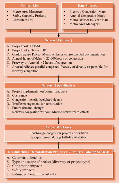
(Source: Federal Highway Administration.)
Use of Data to Identify and Rank Bottlenecks
A wealth of data is available to analysts for bottleneck analysis. Over the last decade, and particularly in the last few years, the transportation industry has experienced increased availability of probe data sources for speed (travel-time) data. The typical arrangement is that companies who resell the speed data have agreements with fleet owners/managers and others to obtain the probe data. Some of these companies also have probe data coming in from navigation devices or smartphone apps—all sources of travel-time information. The "value-add" of these commercial companies is that they aggregate and summarize the speed data based upon their multiple-source probes. Coverage is often comprehensive on higher functional classification roadways (freeways, highway, and major arterials). Typically, vehicle probe data are obtainable in annual summaries for a 15-minute or hourly time period, or more detailed data are available for every predefined time intervals ("epochs") over a long time span (e.g., continuously collected over a year). These data are commonly available at 5 minute or even 1-minute epochs. Some vendors of vehicle probe data can provide truck-specific speed data in a similar format.
An example of a probe data source is the Federal Highway Administration (FHWA) National Performance Management Research Data Set (NPMRDS), which provides travel-time data in 5-minute time aggregations (throughout the year) for both trucks and passenger cars on the traffic message channel roadway network. TMC is the traveler information industry standard roadway network geography used for reporting traveler information.
Intelligent transportation systems (ITS) roadway detectors are another method of speed data collection. These detector technologies represent traditional monitoring equipment used by public agencies to monitor traffic conditions. Typical ITS detector types include:
- Inductive loops.
- Magnetometer.
- Piezoelectric or bending plates (weigh-in-motion).
- Radar.
These technologies all can provide speed, classification and speed data. Piezoelectric or bending plates also can provide weight information. Speeds can be grouped by classification with these detectors (i.e., speeds for a few length-based truck classes are available). Unlike the methods for speed data collection mentioned up to now, ITS roadway detectors may allow for the measurement of speed information by lane.
A key distinction with these technologies is that speeds are obtained "at a point" rather than direct measurement of travel time along the roadway link of interest. To obtain travel time from these speeds, the analyst must convert these speeds to a travel time along the link of interest. One typical way to do this is to assume the point speed is representative across the entire link and to divide the link length by the (point) link speed to obtain a travel time along the link of interest.
Empirical data is highly useful for both identifying a "candidate pool" of potential bottleneck locations as well as for ranking bottlenecks by the severity of the problems. Often this is a two-step process:
- Scan for potential bottlenecks using relatively straightforward methods. Most States have data systems capable of matching traffic volumes with roadway capacity and these can be used to perform the initial scan.
- Perform more detailed analysis using travel time data or more sophisticated modeling methods. Here one wants to produce objective estimates of congestion levels at each of the potential bottlenecks as well as to identify the root cause of the problems. Travel time data from detectors on urban freeways is now widely available through the activities of traffic management centers. Figure 7 is known as a "heat map" of time, duration, and extent of congestion, and shows how these data may be used to identify bottlenecks. Special travel time runs, aerial photography, or video of suspected bottleneck areas can also be used to pinpoint sources of operational deficiencies. Finally, private vendors are constantly improving their probe-derived travel time data that can be used for congestion analysis and bottleneck identification on virtually all highways. "Big data" has had a tremendous impact on the ability to analyze past, present, and even future (predictability) conditions.
Figure 7. Graph. Speed contours over time and space showing bottleneck locations.
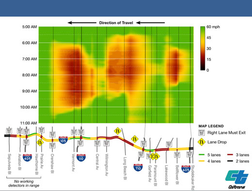
(Source: California Department of Transportation, District 7 Los Angeles, Active Traffic Management (ATM) Congestion Relief Analysis Study, 2005.)
Performance Measures for Bottlenecks
A wide variety of performance measures are available for conducting bottleneck analysis. The starting point for developing these measures is travel time data that is ideally continuously collected. Traffic volume data is also required for a few measures. Some of the more useful measures are:
- Total Delay (vehicle-hours and person-hours): Actual vehicle-hours (or person-hours) experienced in the highway section minus the vehicle-hours (or person-hours) that would be experienced at the reference or "ideal" speed.
- Mean Travel-Time Index (MTTI): The mean travel time over the highway section divided by the travel time that would occur at the reference or "ideal" speed.
- Planning Time Index (PTI): The 95th percentile Travel-Time Index computed as the 95th percentile travel time divided by the travel time that would occur at the reference or "ideal" speed.
- 80th Percentile Travel-Time Index (P80TTI): The 80th percentile Travel-Time Index computed as the 80th percentile travel time divided by the travel time that would occur at the reference or "ideal" speed.
- Hours of Congestion per Year: Number of hours where vehicle speeds are below a pre-set thresholds.
- 95th Percentile Queue Length (uninterrupted facilities): Developed from a distribution of queue lengths, the highway distance where the speeds of contiguous segments upstream of an identified bottleneck location are less than a pre-set threshold.
- Average Queue Length (uninterrupted facilities): Average highway distance where the speeds of contiguous segments upstream of an identified bottleneck location are less a pre-set threshold.
- Amount of delay on the 85th percentile "worst delay day" of the year.
When constructing bottleneck measures, analysts should define segments upstream of the actual bottleneck location for compiling them. Analysts should also be aware that the effects of a bottleneck (queuing) may affect intersecting highways upstream of the bottleneck location.
Analyzing Bottlenecks
Bottleneck analysis is necessary to study not only the subject location, but also the impacts of potential bottleneck remediation on upstream and downstream conditions. The analysis will justify action to correct bottlenecks, confirm the benefits of bottleneck remediation, or check for hidden bottlenecks along a corridor. When conducting bottleneck analysis, care should be taken to ensure that:
- Improving traffic flow at the bottleneck location doesn't just transfer the problem downstream. The existing bottleneck may be "metering" flow so that a downstream section currently functions acceptably, but the increased flow will cause it to become a new bottleneck.
- Future traffic projections and planned system improvements are inclusive in the analysis. Safety merits also should be strongly considered.
- "Hidden bottlenecks" are considered. Sometimes, the queue formed by a dominant bottleneck masks other problems upstream of it. Improving the dominant bottleneck may reveal these hidden locations. It is important to take into account the possibility of "hidden bottlenecks" during the analysis stage.
- Conditions not traditionally considered by models are accounted for. There are several bottleneck conditions, such as certain types of geometrics and abrupt changes in grade or curvature, that can't be analyzed by current analysis tools. Engineering judgment will need to be exercised to identify those problems and possible solutions.
These methods were successfully used to identify bottlenecks in the I‑95 Corridor (Figure 8).
The topic of Volume Ten of the Traffic Analysis Toolbox is on Localized Bottleneck Congestion Analysis, focusing on what analysis tools are available, necessary, and productive for localized congestion remediation. This Federal publication (FHWA-HOP-09-042) discusses when, where, and how to study small, localized sections of a facility (e.g., on/off-ramps, merges, lane drops, intersections, weave, etc.) in cost-effective means. Some chokepoints are obvious in their solution; add a turn lane, widen a stretch of highway, retime a signal, or separate a movement by adding a ramp. However, the solution can often lead to hidden or supplementary problems; hidden bottlenecks, disruptions upstream, or undue influence on abutting accesses, etc. Analyzing localized sections of highway is different from analyzing entire corridors or regions. This document provides the guidance that specifies the choice of analysis tools and inputs necessary to analyze localized problem areas.
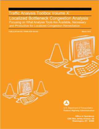
(Source: Federal Highway Administration.)
This document provides the guidance that specifies the choice of analysis tools and inputs necessary to analyze localized problem areas.
A study for the I‑95 Corridor Coalition used private vendor travel time data from INRIX, combined with agency traffic counts, to conduct an analysis of major bottlenecks along the corridor. The study used the data in the following way:
- Scan INRIX data for potential bottlenecks.
- Speeds less than 40 mph for time slice of interest for all of 2009.
- Combine adjacent links.
- Map and identify the physical features that are bottlenecks.
- Interchanges (mainly freeway-to-freeway);
- Bridges; and
- Toll facilities.
- Merge in volumes; compute delay and other performance measures (reliability and queue length).
- Estimate the effect of bottlenecks on long distance trips.
Figure 8. Map. Using vehicle probe data for bottleneck analysis.
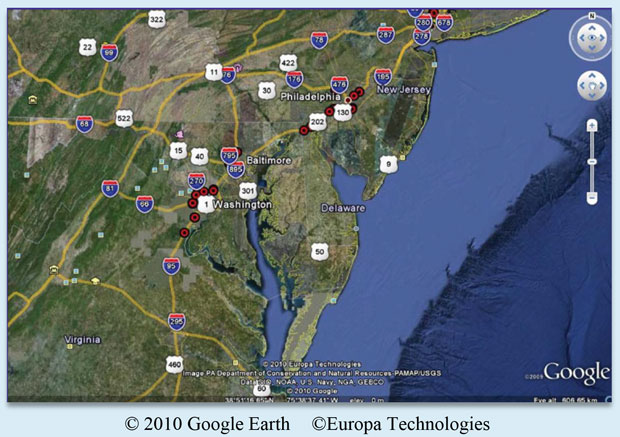
(Source: Federal Highway Administration, Traffic Bottlenecks: A Primer, Focus on Low-Cost Operational Improvements, April 2012.)
Forecasting Bottleneck Performance
A variety of traffic analysis tools are available for forecasting bottleneck performance, but first, future forecasts of demand must be obtained. Once future demand at the bottleneck is obtained, several scales of analysis are possible including:
- Sketch planning (e.g., volume-delay functions).
- Macroscopic analysis (e.g., the Highway Capacity Manual).
- Mesoscopic traffic simulation.
- Microscopic simulation.
FHWA has compiled a comprehensive list of these methods. (Jeannotte, Krista, Andre Chandra, Vassili Alexiadis, and Alexander Skabardonis, Traffic Analysis Toolbox Volume II: Decision Support Methodology for Selecting Traffic Analysis Tools, June 2004.) More recently, the Second Strategic Highway Research Program (SHRP 2) also developed several tools that can be applied (Table 3).
Table 3. Reliability prediction methods developed by the Strategic Highway Research Program 2 program.
| SHRP 2 Project |
Analysis Scale (In Order of Increasing Complexity) |
| L03/C11 |
Sketch planning; system- or project-level. |
| L07 |
Detailed sketch planning; mainly project-level |
| L02 |
Performance monitoring and project evaluations using empirical data. |
| L10 |
Performance monitoring and project evaluations using empirical data. |
| L08 |
Project planning using Highway Capacity Manual scale of analysis. |
| C05 |
Project planning using mesoscopic simulation scale of analysis. |
| C10 |
Regional planning using linked travel demand and mesoscopic simulation analysis. |
| L04 |
Regional planning using linked travel demand and mesoscopic or microscopic simulation analysis. |
| L07 |
Detailed sketch planning; mainly project-level. |
(Source: Federal Highway Administration.)
As an example, SHRP 2 Project C11, Development of Improved Economic Impact Analysis Tools, produced several modules to estimate the economic impact of transportation investments on factors not usually accounted for in transportation analyses: market access, connectivity, and travel-time reliability. It is the reliability module that should be used for sketch planning analysis of truck bottlenecks. A spreadsheet was developed in SHRP 2 Project C11 to estimate the reliability impacts of highway investments. This spreadsheet can be used to estimate the future impacts of truck bottlenecks as it includes the effects of demand, capacity, and incident characteristics. It produces estimates of delay and the distribution of travel-time indices, which indicate reliability performance. It also produces cost estimates for the travel-time savings affected by improvements.
Recent Advances in Data and Analytics for Bottleneck Assessment
Overview
A 2015 research project undertaken by FHWA, Traffic Bottlenecks: Identification and Solutions (FHWA-HRT-16-064), extended earlier work on bottleneck identification and analysis. (Hale, David et al., Traffic Bottlenecks: Identification and Solutions, FHWA-HRT-16-064, November 2016.) This effort developed practical methods for prioritizing and mitigating traffic bottlenecks. A data-driven congestion and bottleneck identification software tool was created that produced numerous performance measures.
Diagnostics
This study also used "heat maps" as a first-cut diagnostic tool to identify the general scale of a bottleneck. A heat map is simply a plot of conditions over time and space for a single time period. This research extended that concept into a "spatiotemporal matrix" (STM) which is a heat map shown for a long time period. Figure 9 shows the idea behind an STM. Each of the "cards" in the deck represent congestion on a given day. Over time, the congestion pattern changes due to the influence of varying demand, weather, work zones, and incidents, as represented by the full deck of cards. Considering the history of congestion over time brings reliability in focus.
Figure 9. Matrix. Spatiotemporal Traffic Matrix (STM).
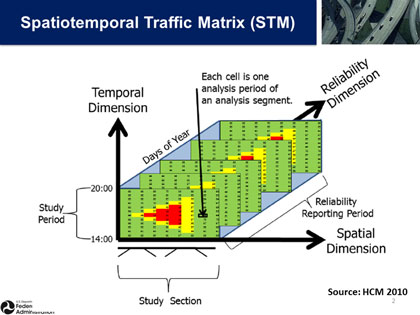
(Source: Federal Highway Administration, Highway Capacity Manual 2010.)
The D.I.V.E. Framework for Defining Bottleneck Performance Measures
The research produced a useful framework for ensuring that a full suite of performance measures is created for bottleneck analysis: D.I.V.E., or duration, intensity, variability, and extent.
- Duration: The amount of time that breakdown conditions persist before returning to an uncongested state (example: average number of minutes a facility is congested every day).
- Intensity: The relative severity of breakdown that affects travel that relate the different levels of congestion experienced on roadways (example: volume-to-capacity ratio).
- Variability: The changes in breakdown conditions that occur on different days or at different times of day (example: reliability measures such as the Planning Time Index (PTI)).
- Extent: The number of system users or components (e.g., roads, bus lines, etc.) that are affected by the bottleneck (example: annual hours of delay).
The research developed a tool for assisting analysis: the Congestion and Bottleneck Identification (CBI) tool. The CBI software tool was developed for this project. The CBI tool can draw an STM for any day of the year. It can also draw an STM for "percentile" days of the year, according to certain performance measures (e.g., the day having the 85th percentile worst bottleneck intensity). Researchers applied California's vehicle-hours of delay conversion, to convert bottleneck speeds into bottleneck delays.
The tool uses two primary performance measures to conduct comparative analyses of bottlenecks: total vehicle delay and the Bottleneck Intensity Index (BII), the delay level below which 85 percent of the total delay exists. The study developed a graphic called the Annual Reliability Matrix (ARM) which shows both intensity (total delay) and variability (reliability as measured by the BII) on a single graphic. Finally, a wavelet method for signalized arterials was added to the tool, to filter out delays that are unrelated to congestion.
Figure 10. Chart. Using the variability in delay to prioritize bottlenecks.
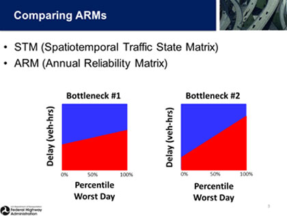
(Source: Federal Highway Administration.)
The CBI tool is useful for comparing and ranking traffic bottlenecks. For example, consider the two bottlenecks in Figure 10. The red area shows the delay for each location; total delay (the amount of red shaded area) is the same for each one. A traditional analysis would indicate that they would receive the same priority. However, by tracking the percentile "worst day" we can see that Bottleneck #2 is subject to much more variability in conditions, Therefore, Bottleneck #2 should be ranked as the higher priority, because more time would be needed to ensure an on-time arrival. That is, the amount of unreliable travel is higher for Bottleneck #2. Essentially, what this approach does is to assess bottlenecks in terms of both total delay and the variability in delay.