Behavioral/Agent-Based Supply Chain Modeling Research Synthesis and Guide

CHAPTER 2. SUPPLY CHAIN MODELING NEEDS AND CONCEPTS

FREIGHT MODELING NEEDS

Travel models are analytical tools designed to provide quantitative input to help answer questions that arise during the policy and planning decision-making process. In the past, many transportation agencies were faced with relatively simple questions, such as how best to allocate highway construction funding to provide capacity in their study area for expected growth in vehicular travel. As agencies are faced with more complex policy and planning questions, the complexity of travel models has increased to provide the necessary level of detail and policy sensitivity. Passenger travel modeling has led the way in recent years with the gradual transition from trip-based models to activity-based (AB) models among larger agencies in the United States. Freight modeling is undergoing a similar transition to answer increasingly complex freight transportation-related policy questions faced by agencies.

The agencies that participated in this synthesis expressed the need to answer questions posed as part of their planning processes that were beyond the capabilities of their traditional trip-based freight and truck modeling tools. For example, the following policy analysis needs and issues were identified as reasons for implementing a supply chain freight model:

• Understand the economic impacts of freight and the relationship between changes in the economy and changes in demand for freight transportation:
  • Address the economic impacts of freight transportation-based changes in the economy and freight delivery systems.
  • Explain economic choices made for goods movement across multiple modes and commodities.
  • Provide a picture of the study area's role in the national freight economy, including the economic competitiveness of the study area compared to other areas.
  • Understand the effects of the evolution of industry in the study area (transition to emerging industries such as aerospace, clean energy, life sciences, and creative industries).
  • Understand the connections between the economy of the study area, the resulting demand for freight movement, and the performance of the transportation system in a complex and congested region.
  • Develop freight forecasts that are responsive to changes in economic forecasts, changing growth rates among industrial sectors, and changing rates of economic exchange and commodity flows between sectors.
  • Provide inputs regarding how freight transportation will contribute to economic recovery.
  • Evaluate technological shifts in logistics and supply chain practices (e.g., near-sourcing, outsourcing, productivity enhancements).
• Understand the relationships between freight movement and land-use and spatial development in a study area:
  • Increase understanding of freight-generating industrial and commercial development and how these land uses relate to goods movement, including first and last mile.
  • Deliver insight into how land use, local economic development and demographic factors drive freight movement, trip generation, and freight demand analysis.
  • Incorporate the evolution of land-use patterns in freight-related industries, such as increased development of intermodal logistics hubs and larger regional distribution centers.
• Understand current freight movements in a study area:
  • Provide an understanding of how freight currently moves throughout the study area.
  • Provide an understanding of truck touring for urban goods delivery and service trips.
  • Represent long-distance truck movements and empty truck movements.
• Evaluate complex freight-related policies and freight-related infrastructure improvements:
  • Evaluate the transportation impacts of freight policies such as overnight delivery ordinances or the expansion of logistics terminals within the region.
  • Anticipate the effects of freight-related government and private sector decisions that affect the transportation system and its uses.
  • Evaluate the local freight distribution system, the impacts of port expansions, and improvements to intermodal facilities.
  • Support comprehensive analysis of infrastructure needs and policy choices pertaining to the movement of goods.
  • Provide a freight forecasting model for an extensive and complex study area that includes the operations of several significant industries with connections to major freight ports and the U.S. border.
• Understand the environmental impacts of freight and truck movements.
  • Develop more detailed network assignments by truck type to support environmental analysis.

• In most cases, the freight models used by agencies in this report were designed to support the needs of multiple stakeholders in large and complex regions, which added to the diversity of policy needs and issues. For example, several of the freight models were designed to cover megaregions with multiple Metropolitan Planning Organizations, or large single-Metropolitan Planning Organization regions, or were jointly developed by State and regional agencies. In several cases, modal agencies, such as port authorities, were involved in the development of the freight models. This expansion beyond a more historically typical highway-focused use of travel models added to the need to cover all freight transportation modes rather than, for example, a truck-only model.

Table 1. Summary of Freight Modeling Needs, by Type.

Type	Economic Forecasts	Growth Rates by Industry	Logistics Practices	Roadway Congestion	Private Sector Operations	Logistics Terminals	Ports	Truck Volumes
Economic Impact	✓	✓	✓	✓	✓	✓	✓
Land Use		✓			✓	✓	✓
Policies	✓	✓	✓			✓	✓
Infrastructure				✓		✓	✓	✓
Environmental				✓	✓	✓	✓	✓

Table 1 summarizes agencies' freight modeling needs, by type. This demonstrates what elements of freight modeling needs influence the five categories of need (economic impact, land use, policies, infrastructure, and environmental).

COMMON MODELING METHODS

Approaches to freight travel demand modeling in the United States range from conventional four-step planning models to more advanced integrated supply chain, economic-based, and tour-based models. This synthesis describes the experiences of public agencies in the United States with advanced supply chain freight travel demand modeling.

The traditional four-step freight demand modeling approach is defined by its four sequential stages of trip generation, trip distribution, modal split, and traffic assignment. In these models, the demand modeling process is aggregate and trip-based or commodity-based with limited analysis of individual trip behavior.

Four-step models are relatively weak in terms of behavioral foundation, which often leads to limited model capabilities and model accuracy issues. These models fail to model the underlying economic behaviors from which the demand is derived. The main drawback of these aggregate models is their inability to capture the complexity of freight policy systems and their failure to replicate the supply chains and logistics decisions made by individual players in the freight supply chain.

To address some of the limitations mentioned above, advanced freight demand forecasting models have been proposed. These advanced models are disaggregate models that incorporate supply chain procedures or truck touring aspects. Disaggregate freight models can also provide more capabilities than aggregate models to evaluate policies and investments.

The following text describes common components/approaches to advanced supply chain modeling, including firm synthesis, buyer-supplier matching, distribution channel and vehicle choice, shipment size, mode choice, and truck touring models. Figure 2 shows a supply chain modeling process.

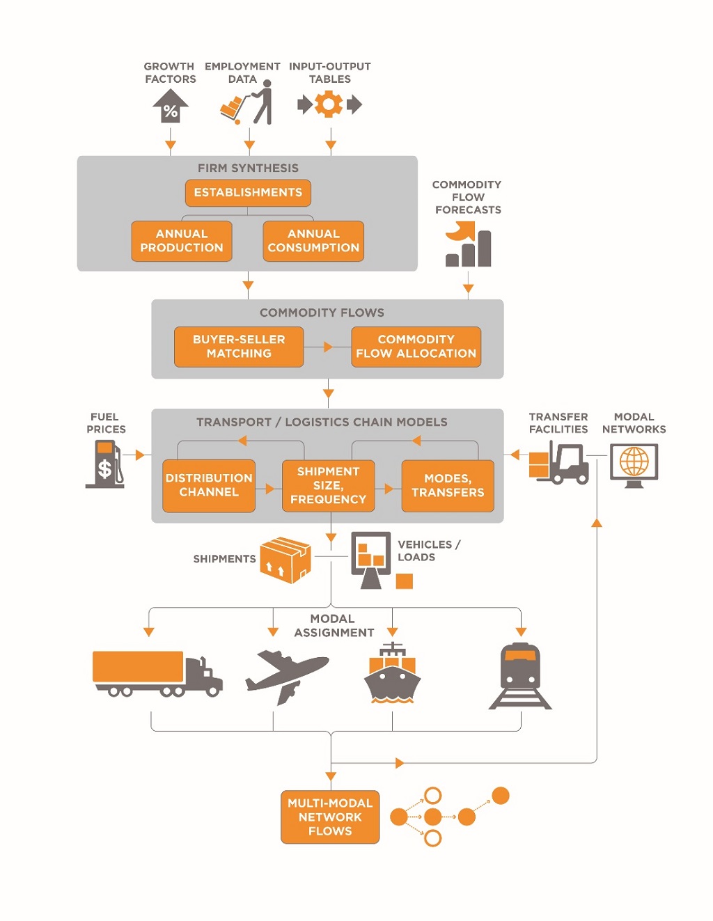
Figure 2. Behavioral Supply Chain Modeling Process.
Source: RSG (2016)

Firm Synthesis

In behavioral-based supply chain freight models, the first step is firm synthesis—the process of creating individual firm objects to represent establishments and replicate their freight movement and travel behavior. This process uses employment data for the modeling region, which may be available in different forms, to assemble a record of establishments with location, size, industry, production, and consumption information. For a fully disaggregate approach, the ideal form of data would be an employment database with records for individual establishments. These records would include addresses for physical locations, number of employees, and detailed NAICS industry and commodity codes. Employment databases with this level of detail are produced by commercial vendors, such as InfoGroup, and can be acquired for a fee; however, they may not be comprehensive in their coverage of all industry sectors, such as agriculture, construction, public administration, and self-employed individuals and small businesses.

Publicly available datasets include the Longitudinal Employer-Household Dynamics (LEHD) and County Business Patterns (CBP) datasets, both published by the U.S. Census Bureau. These datasets are discussed in the next section.

The process by which these more-aggregate datasets are transformed into synthetic firms for simulation modeling is relatively straightforward, and depends on the level of aggregation in the data and the desired level of disaggregation for the model. The basic steps are as follows:

1. Develop joint distributions of the number of establishments by NAICS codes and employee-size groupings. Start with the most disaggregate groupings of NAICS (e.g., six digits for CBP) and establishment size available in the source data, and aggregate as necessary to the groupings needed for the model. (Aggregation at the county level is typical for LEHD or CBP.)
2. Enumerate establishments. Create an establishment record/object for the simulation (enumeration) for each count of an establishment by establishment size and category. This should provide both a NAICS code attribute and an establishment-size attribute. If locational attributes are needed for a finer geographic resolution than the county, then distribute the synthesized establishments to traffic analysis zone or similar geography using local employment data. If commercial employment data are available, then use these data to create synthetic establishments in more-precise geographic locations.
3. Add production. The Make tables (commodities that are produced by each industry) from an Input-Output (IO) account are used to estimate the dollar value of commodities produced by synthetic establishments, differentiated by industry and establishment size. For some industries that produce multiple commodities, one approach is to select a single production commodity. This permits estimation that the amount produced is proportional to the establishment size. This can then be done for all establishments in the United States that produce that commodity domestically, which can also be derived from the Make table. Generally, selecting more than one commodity will significantly increase the computational and memory requirements.
4. Add consumption. The IO Use or Direct Requirements table can generate consumption commodities using a production commodity and quantity. The Direct Requirements table shows the dollar amount of each input commodity needed to produce a dollar of the output (production) commodity. Because most production commodities use scores of input commodities, simplifying assumptions may be necessary to limit the number of modeled input commodities to a manageable number (and possibly rescaling total quantities to ensure adequate representation of flows).

Following these steps produces a list of establishments with location, establishment size, industry, production, and consumption details that aggregate to meet the joint distributions of establishments by industry and establishment size.

Allocation of Freight Demand

Buyer-Supplier Matching

The relationships between buyers and suppliers, who ultimately become shippers and receivers of commodities, is the next core step of the behavioral-based supply chain freight models. Buyers evaluate characteristics of suppliers and transportation costs to select supplier establishments to transport goods. This process emulates the business decision to select a supplier to allocate freight demand between buyers and suppliers. The approach of buyer-supplier matching retains aggregate-level controls at the level of the Freight Analysis Framework (FAF) zone, county, or other regional geographic unit, while allowing simulation of freight movements at the subregional level by synthesizing establishments and simulating the matching of buyers and suppliers. The buyer-supplier matching process follows four steps:

1. Generate an annual production quantity as a function of establishment size (employment) for each synthetic establishment that is a producer of a commodity.
2. Generate the purchase requirements of input commodities for each synthetic establishment producing a forecasted quantity of commodity using IO accounts tables.
3. Choose a supplier located in a zone that produces that commodity for each input commodity to be purchased.
4. Allocate the commodity flow amount to buyer-supplier pairs in each zone, in proportion to their probabilities, for each FAF zone-to-zone commodity flow value.

To apply the supplier firm selection model (Figure 3), the model creates a choice set of suppliers for each buyer firm based on the commodities it requires and the corresponding NAICS code of the suppliers. A supplier firm is excluded from the choice set if no flows for the commodity being traded are observed in the FAF dataset between the relevant FAF zones. Great circle distances (GCDs) are based on the buyer and supplier FAF zones. The model calculates a score for each buyer and potential supplier pair using the attested coefficients and adding a random value for stochasticity. For each buyer firm, the model selects the supplier firm with the best (highest) score.

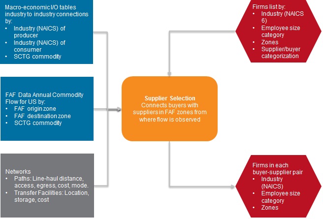
Figure 3. Supplier Firm Selection Model Process.
Source: (RSG, University of Maryland, and Vision Engineering and Planning, 2017)

Commodity Flow Allocation

The commodity flow allocation process predicts the demand in tonnage for shipments of each commodity type by each business establishment in each industry. The demand is developed to represent the goods produced by each business establishment and the goods consumed by each business establishment that leads to a freight shipment to, from, or within a region. The commodity flow allocation model's primary inputs are the FAF freight flows and the buyer-supplier pairs simulated in the supplier firm selection model. The model uses the consumption requirements by business establishments of different industries calculated in the firm synthesis model to determine the allocations between industry types. The amount of commodity shipped on an annual basis between each pair of firms is apportioned based on the number of employees at the buyer and their industry so that observed commodity flows are matched.

Figure 4 shows the commodity flow allocations model's inputs and outputs. Once buyer and supplier pairs have been established, the annual flow between each of the pairs is estimated, the FAF dataset is used to apportion goods demand to each buyer-supplier pair based on the size of the buyer business establishment. An estimate of consumption (of the commodity being consumed) by a buyer business establishment is calculated based on the value (in dollars) consumed per employee, which is obtained using processed IO economic tables. The values consumed per employee are calculated for each combination of supplier-buyer industry NAICS from the IO tables.

Figure 4. Commodity Flow Allocation Model.
Source: (RSG, University of Maryland, and Vision Engineering and Planning, 2017)

The values consumed per employee are used to calculate a consumption estimate (in dollars) for each buyer business establishment. A share of consumption for each business establishment in a particular zone is then calculated based on the consumption estimate. These shares are used to apportion freight flows for each commodity into a zone for individual buyer firms. This results in an estimate of annual goods demand between each of the buyer-supplier pairs.

Transportation Logistics Chain Models

Distribution Channels

The distribution channel model component selects the distribution channel for the shipment, a key element of the framework that represents an important business decision made by shippers. A distribution channel refers to the supply chain a shipment follows from the supplier to the consumer/buyer, which is critical to freight-related business operations. The supplier firms may use their own transportation resources or send shipments to the buyer using third-party logistics (3PL) firms. The distribution channel might affect the cost, shipment size, and frequency of shipments between a buyer-supplier firm pair. In this framework, the transfer facilities are represented in the supply chain rather than including all establishments that goods move through as they travel from the producer to the consumer; this is because of limited data for these detailed supply chains. The distribution channel model uses discrete choice methods to identify the unique aspects of the supply chain.

The concept of distribution channel can be simplified to obtain a reasonable sample for model estimation, as shown in Figure 5. Four alternatives for distribution channels are: direct, one-stop type, and two-stop type; and three-stop types, where stop type is a warehouse, distribution center, or consolidation center. Distribution channels that involved only one warehouse stop, or only one distribution center stop, are considered the same. Future datasets may allow for including more complex representations of distribution channels.

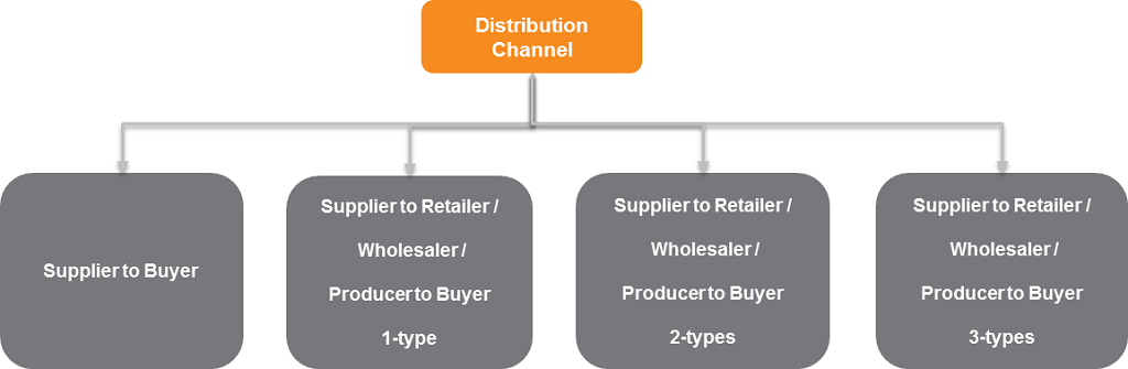
Figure 5. Distribution Channels.
Source: (RSG, University of Maryland, and Vision Engineering and Planning, 2017)

Figure 6 shows a schematic of the distribution channel model. The distribution channel model simulates shipments between all the buyer-supplier pairs based on the type of commodity. The manufactured goods model is applied for all commodities other than food. At this stage in the framework, the unit of analysis is shipments by all modes; therefore, the distribution channels are not mode specific and may be completed by a single mode or be multimodal (the process of selecting modes for movement of each shipment takes place in the mode and transfer model).

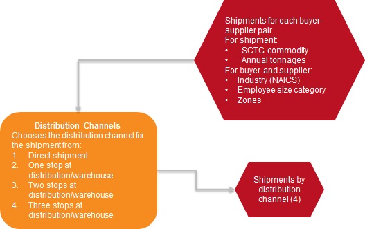
Figure 6. Distribution Channel Model Process.
Source: (RSG, University of Maryland, and Vision Engineering and Planning, 2017)

Shipment Sizes

In the shipment size model component, the annual goods flow between buyer-supplier pairs is broken down into individual shipments. The shipment size (weight) and the corresponding number of shipments per year are determined. Shipment size affects the mode used to transport the shipment. A multinomial model is estimated for choice of shipment size. A vehicle survey dataset is used for estimating the discrete choice model. The Texas commercial vehicle survey is a commonly used dataset due to its relatively high sample size. The distribution channel typically influences the choice of shipment size. Stop-level data were transformed into tour-level data and the distribution channel is assigned based on the stops made by the truck at ports, intermodal facilities, warehouses, and distribution centers. Figure 7 illustrates the shipment size and frequency model. The shipment size choice is simulated for all the buyer-supplier firm pairs using the estimated models.

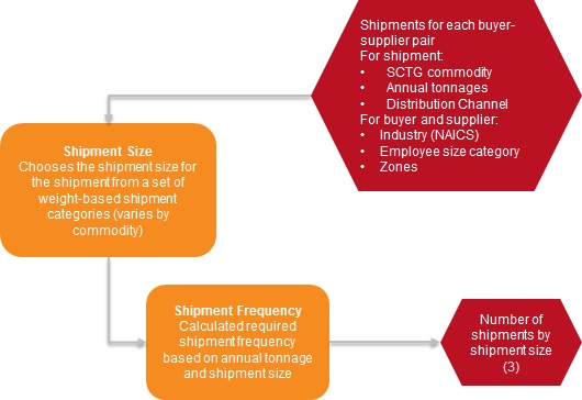
Figure 7. Shipment Size and Frequency Model Process.
Source: (RSG, University of Maryland, and Vision Engineering and Planning, 2017)

Modes and Transfer

The mode and transfer step assigns a mode for shipments transported between each buyer-supplier pair. Four primary modes (road, rail, air, and water) are typically included in the mode choice model. Pipeline can be added as a fifth mode if significant in any area. The modes and transfer locations on the shipment paths are determined based on the travel time, cost, characteristics of the shipment (e.g., bulk natural resources, finished goods), characteristics of the distribution channel (e.g., whether the shipment is routed via a warehouse, consolidation, or distribution center), and whether the shipment includes an intermodal transfer (e.g., truck-rail-truck). A two-step process selects a mode and path (from a set of feasible modes and paths)—one that would have the least annual transport and logistics cost using a two-step process:

1. Enumerate a set of feasible paths between each origin-destination pair.
2. Apply a reasonable set of parameters to the path skims to generate total annual transport and logistics costs for each combination of path and mode.

In calculating the total annual costs for each pair of seller and buyer, supply chain and inventory control costs are considered and incorporated to account for the inventory-associated costs. Methods developed by de Jong and Ben-Akiva (2007) can be used to predict the path and mode of long-haul movements of freight. The path includes identifying the location of intermodal transfer facilities, distribution centers, or warehouses are shipments are consolidated or deconsolidated. Detailed networks of road and rail for the United States were used, in addition to networks describing airport and port locations, domestic waterway connections, and GCDs between airports and between ports and international destinations. The total logistics cost that the buyer and supplier encounter is the sum of transport and inventory costs and can be itemized as shown below:

This formulation simulates logistics decisions in a joint fashion by capturing transport and logistics costs in a single equation. This effectively reflects the real-world decision-making of freight movers by accounting for different components of costs. Figure 8 shows a schematic of the mode and transfer choice model. The buyer-supplier pairs dataset now has information on buyer firm ID, supplier firm type ID, commodity type (SCTG), annual flow in tons and dollars, distribution channel, and the shipment size. Modal skims developed are merged into the buyer-supplier pairs dataset.

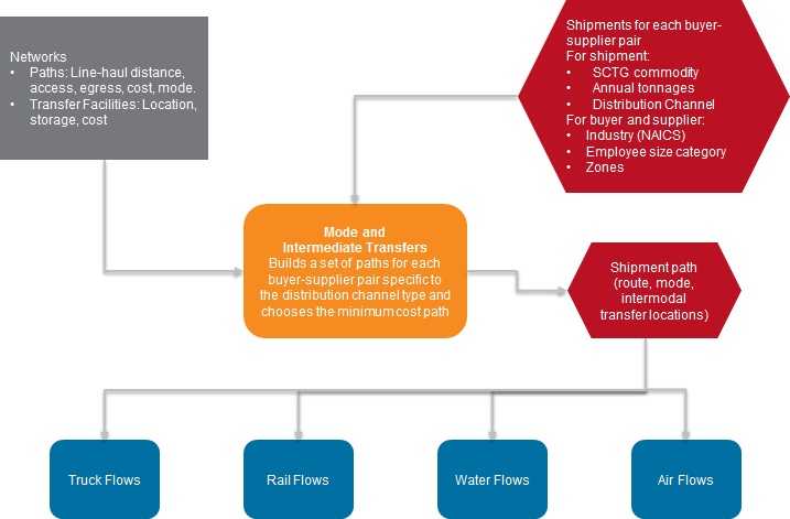
Figure 8. Mode and Intermediate Transfer Model Process.
Source: (RSG, University of Maryland, and Vision Engineering and Planning, 2017)

TOUR-BASED TRUCK MODELS

The behavioral-based supply chain freight model can be integrated with a regional truck touring model, which is a sequence of models that takes shipments from their last transfer point to their final delivery point. The integrated modeling system connects the national supply chain models with the regional truck touring models. The final transfer point is the last point at which the shipment is handled before delivery (i.e., a warehouse, distribution center, or consolidation center for shipments with a more complex supply chain or the supplier for a direct shipment). It performs the same function in reverse for shipments at the pick-up end, where shipments are taken from the supplier to distances as far as the first transfer point. For shipments that include transfers, the tour-based truck model accounts for the arrangement of delivery and pick-up activity of shipments into truck tours.

A commercial services touring model can be developed to provide a comprehensive representation of all trucks. This model has the same structure and features of the regional truck touring model, but demand is generated from businesses and households in the region rather than from goods movement. These commercial services include utilities, business, and personal services. Delivery of goods to residences by parcel delivery are typically included in the services touring model.

The model produces trip lists for all the freight delivery trucks and commercial vehicles in the region that can be assigned to a transportation network. The truck touring model components predict the elements of the pick-up and delivery system within the region through several modeling components, as shown in Figure 9:

1. Vehicle and tour pattern choice. Predicts the joint choice of whether a shipment is delivered on a direct or a multistop tour and the size of the vehicle that makes the delivery.
2. Number of tours and stops. Predicts the number of multistop tours required to complete all deliveries and estimates the number of shipments that the same truck delivers.
3. Stop sequence and duration. Sequences the stops in a reasonably efficient sequence but not necessarily the shortest path. Predicts the amount of time taken at each stop based on the size and commodity of the shipment.
4. Delivery time of day. Predicts the departure time of the truck at the beginning of the tour and for each subsequent trip on the tour.

The output from the truck touring model can be integrated with a regional passenger travel model for highway assignment and then become part of the regional travel demand modeling system.

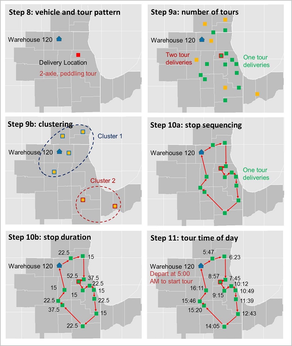
Figure 9. Truck-Touring Model Steps.
Source: (Smith, 2013)

MODEL APPLICATIONS

Behavioral-based supply chain freight models can be used for myriad policy applications. These are dependent upon the specific components that are included and can be categorized into two main types of modeling systems: 1) national supply chain models; and 2) regional truck touring models. The national supply chain models include the firm synthesis, allocation of freight demand, and transportation logistics chain components and can support the following policy analyses:

• Modal alternatives. There is direct competition between air, rail, water, and truck for freight movements, and any infrastructure investments being considered should be evaluated in the context of this competition. These alternatives are evaluated nationally and—to a lesser degree—internationally to capture any impacts in a State or region.
• Pricing. Many aspects of pricing can and should affect statewide freight forecasts. Pricing can be a strategy to manage demand or raise revenues (e.g., toll roads, gas taxes, mileage fees). Pricing affects the travel decisions of drivers, shippers, carriers, and 3PL establishments differently.
• Economics. Policies to improve economic conditions will affect freight and goods movement. Economic conditions could be tested by adjusting these inputs to understand the effects on freight mobility of a greater demand for goods. Higher employment in a State will lead to additional production and consumption of commodities, which can be represented by alternative employment and commodity flow inputs. Policies such as freight tolling and truck restrictions can be analyzed to understand the effects on freight.
• Environmental. Policies to reduce transportation-related emissions can have effects on freight and goods movement. An increase in the gas tax will influence gas consumption and potentially reduce vehicle miles traveled. Carbon taxes may also affect the cost of freight transport. The Environmental Protection Agency may change fuel standards for trucks, which would affect the transport cost for trucks.
• Safety. Policies such as driver hours-of-service regulations and technologies to reduce accidents for hazardous materials transport will affect decisions on the cost to transport goods and on what modes to use for certain goods.
• Airport, Seaport, or Rail Planning. Policies made by airports, seaports, or rail operators regarding new capacity, intermodal terminals, or environmental effects can be evaluated.

Regional truck touring models can address regional impacts for the following policy analyses:

• Policies. Regional policies such as taxes, tolls, or local delivery times will result in different freight mobility in different cities. Truck route restrictions and truck size and weight limits can also affect route decisions.
• Environmental. Policies to reduce regional emissions impacts can be evaluated in a similar manner as the national supply chain models (see preceding description).
• Pricing. Regional pricing options can be evaluated in a similar manner as the national supply chain models (see preceding description).
• Airport, Seaport, or Rail Planning. Regional infrastructure for ground access to ports or rail stations can be evaluated.

The project team identified several model applications in the case studies, including the following:

• Inform infrastructure investment decisions.
• Evaluate congestion on highways.
• Test the effectiveness of transportation policies on mobility and the economy. This will include policies such as freight tolling and truck restrictions. This will also include evaluating economic scenarios.
• Produce multimodal system performance measures for freight.
• Evaluate the effects of private sector decisions on the transportation system.
• Provide regional agencies with intercity freight travel information for regional planning purposes.
• Evaluate freight mobility alternatives for long-range plan development and corridor analyses.
• Consider truck emissions in federal transportation conformity determination.
• Evaluate accessibility to manufacturing and industrial centers.
• Assess emergency management and evacuation procedures.