Active Transportation and Demand Management (ATDM) Analytical Methods for Urban Streets
CHAPTER 4. SYSTEM PERFORMANCE MEASUREMENT
This chapter presents the potential traffic performance measures for evaluating active transportation and demand management (ATDM) impacts. Results of the Task 5 – System Performance Measures review were documented in a detailed technical memorandum in February 2016, and are repeated here in this chapter. The first section of the chapter summarizes the available performance measures from existing and known data sources, collected during Task 4, which focused on before- and-after assessment of ATDM strategies. The second section summarizes the "Performance Measures (Measures of Effectiveness) for ATDM Analysis" section of the 2013 Federal Highway Administration (FHWA) report, entitled: "Guide for Highway Capacity and Operations Analysis of Active Transportation and Demand Management Strategies" (Dowling, Margiotta, Cohen, & Skabardonis, 2013). The 2013 study focused primarily on freeways, but many of the performance measures suggested by that study could ultimately benefit the urban streets ATDM study. In the third section, additional performance measures used in the current Analysis, Modeling and Simulation testbed project are listed. Some of these performance measures would be generated by the simulation experiments in Task 6. The fourth section summarizes performance measures that can be generated by two of the available software platforms for Highway Capacity Manual
(HCM) urban street reliability analysis: Streetval-Java, and HCS-Streets. If the macroscopic before- and-after ATDM impacts found during Task 6 can be successfully coded into one or both of these platforms, it could become possible to assess ATDM impacts in terms of annual reliability and other advanced measures.
ADAPTIVE SIGNAL PERFORMANCE MEASURES
Virginia Department of Transportation (VDOT) Study (InSync)
Crow Canyon Road and Bollinger Canyon Road in San Ramon, California:
- Fifty percent decrease in average travel time during the PM peak, in the major-street direction.
- Unspecified increase in travel time and approach delay PM peak, off-peak direction.
- Seventy-five percent decrease in average major approach delay during the PM peak.
- Average delay along minor streets increased by approximately 3 seconds per vehicle.
10th Street Corridor in Greeley, Colorado:
- Nine percent decrease in travel times.
- Thirteen percent decrease in stopped delay.
- Eleven percent increase in average speed.
- Six percent decrease in fuel consumption and emissions.
- Forty-five percent decrease in stops.
- Side street delays increased on some approaches.
Original Research:
- No benefits when conditions are oversaturated.
- Twenty percent reduction in stops.
- Seven percent increase in average speed.
- Seven percent decrease in travel time.
- Side street delays increase by 5-10 sec/veh.
- Adaptive signal control technology (ASCT) most effective at sites with variable traffic demands (e.g., seasonal variations, school schedules, incidents, special events).
- ASCT not effective on routes with high truck volumes.
- Long signal spacing will reduce ASCT effectiveness.
- ASCT improves mainline operations if the corridor does not have traffic or geometric characteristics that impair progressive flow.
- ASCT improves mainline operations if corridor does not already operate at a good level of service (LOS).
Based on these VDOT study results, the team concluded that sensitivity analysis in the ATDM project should examine: degree of saturation, variable traffic demands, percent trucks, signal spacing, progression quality, non-recurring events (e.g., weather, incidents), and cycle lengths.
Cornell Road Study (InSync)
- Fourteen percent decrease in travel times.
- No improvement in average delay.
- Ten to twenty second increase in cycle lengths.
Non-Recurring Conditions VISSIM Study (InSync)
- ASCT advantages are more significant for nonrecurring traffic conditions (e.g., weather, incidents, rail pre-emption).
- Sixteen percent decrease in network-wide average delay (no non-recurring events).
- Nine percent decrease in network-wide stops (no non-recurring events).
- Seven percent decrease in network-wide travel time (no non-recurring events).
- Twenty-four percent decrease in network-wide average delay (with non-recurring events).
- Twelve percent decrease in network-wide stops (with non-recurring events).
- Twelve percent decrease in network-wide travel time (with non-recurring events).
Powell Road Study (SCATS)
- One percent decrease in 24-hour travel times.
- Seven percent decrease in midday travel times (9 am – 2:30 pm).
- Two percent increase in pm peak travel times (2:30 pm – 7:00 pm).
- Six percent increase in overnight travel times (12:00 am – 5:30 am).
- No change in am peak travel times (5:30 am – 9:00 am).
- No change in evening travel times (8:00 pm – 12:00 am).
Redmond Road Study (SCATS)
- Twelve percent decrease in major-street travel times.
- Twenty-six percent decrease in major-street travel times during the county fair.
- Five to twenty second increase in cycle lengths.
- No change in the buffer index.
- Two-second decrease in average delay per vehicle.
- Fifteen-second decrease in average delay per vehicle during the county fair.
Tualatin-Sherwood Road Study (SCATS)
- No change in the buffer index.
- Ten to fifteen 1 second increase in cycle lengths.
- Fifty-second decrease in travel times (over 1.3 miles) during high-demand periods.
- Ten-second increase in travel times (over 1.3 miles) during low-demand periods.
REVERSIBLE CENTER LANE PERFORMANCE MEASURES
Salt Lake City Flex Lanes
Vehicle trips and travel times were measured in the field.
Intersection delays were computed by an un-named traffic model.
- During the PM peak period, westbound (peak direction) travel times were reduced by 50 seconds and eastbound (non-peak direction) were reduced by 20 seconds.
- During the AM peak period, eastbound (peak direction) travel times were reduced by 45 seconds, but increased in the westbound direction (non-peak direction) by 65 seconds.
- The benefits of the travel time savings in both the AM and PM peak directions (which have significantly higher traffic volumes) outweigh the detriments of the increased travel time in the AM non-peak direction.
- Traffic volumes on 5400 South increased during Flex Lane operations (AM and PM peak periods) in the peak direction.
- At one of the two data collection locations, traffic volumes decreased during Flex Lane operations (AM and PM peak periods) in the non-peak direction. The other data collection location showed an increase in PM traffic volumes while AM traffic volumes remained the same.
- The Flex Lanes currently save a total of $792,000 in user costs per year (based on travel time savings).
- The Flex Lanes currently reduce idle emissions by 1.24 tons per year.
DYNAMIC LANE GROUPING PERFORMANCE MEASURES
Bottleneck Project (Saxton Transportation Operations Laboratory Task Order 6) Study
Study Synchro ™ datasets were provided by Randy Dittberger (VDOT) for two signalized corridors in Northern Virginia. These datasets are used "to store signal timings," but were not calibrated for local conditions. Intersection delays were computed by SimTraffic™.
Out of 17 intersections, three were identified as top candidates for dynamic lane grouping:
- Colts Neck Road and Sunrise Valley Drive, with a 32 percent reduction in intersection-wide average delay per vehicle.
- Nutley Street SW and Lee Highway, with a 23 percent reduction in intersection-wide average delay per vehicle.
- Reston Parkway and Sunrise Valley Drive, with a 10 percent reduction in intersection-wide average delay per vehicle.
The third intersection derived benefits from dynamic lane grouping (DLG) treatment at Colts Neck, due to its close proximity; specifically, queue spillback was reduced. Due to the lack of sufficient field data, HCM-compatible models for DLG would be heavily dependent on software modeling, to be performed during the Original Research task. Although some researchers developed mathematical programming models for optimizing the effects of DLG (Zhang & Wu, 2012) (Zhao J., Ma, Zhang, & Yang, 2013), these models were not developed with HCM compatibility in mind.
SUMMARY OF TASK 4 PERFORMANCE MEASURES
Figure 9 summarizes a set of nine performance measures from available data sources. These performance measures were relevant to the three chosen active traffic management (ATM) strategies for this project. The amount of available data in Figure 9 leads to the conclusion that more data would be needed, to confidently development HCM models. However the available data succeed in demonstrating potential benefits of the strategies, and provide a benchmark for the simulation studies in Task 6 – Original Research.
Figure 9. Chart. Summary of nine performance measures from existing data sources.
| Source |
ASCT |
Reversible |
DLG |
Time Period |
Spatial |
Travel Time |
Delay |
Emissions |
Stops |
Speed |
Volumes |
Cycle Length |
Buffer Index |
User Costs |
| California |
InSync |
 |
|
pm peak |
major-street |
-50% |
-75% |
|
|
|
|
|
|
|
| California |
InSync |
|
|
pm peak |
minor-street |
|
3% |
|
|
|
|
|
|
|
| Colorado |
InSync |
|
|
pm peak |
major-street |
|
-13% |
|
|
|
|
|
|
|
| Colorado |
InSync |
|
|
pm peak |
minor-street |
|
3% |
|
|
|
|
|
|
|
| VDOT |
InSync |
|
|
|
|
-7% |
|
|
|
|
|
|
|
|
| VDOT |
InSync |
|
|
|
minor-street |
|
+7 s/veh |
|
|
|
|
|
|
|
| VDOT |
InSync |
|
|
oversaturated conditions |
oversaturated conditions |
no benefits |
no benefits |
no benefits |
no benefits |
no benefits |
n/a |
n/a |
no benefits |
no benefits |
| VDOT |
InSync |
|
|
high truck volumes |
high truck volumes |
no benefits |
no benefits |
no benefits |
no benefits |
no benefits |
n/a |
n/a |
no benefits |
no benefits |
| VDOT |
InSync |
|
|
long signal spacing |
long signal spacing |
no benefits |
no benefits |
no benefits |
no benefits |
no benefits |
n/a |
n/a |
no benefits |
no benefits |
| VDOT |
InSync |
|
|
little progressive flow |
little progressive flow |
no benefits |
no benefits |
no benefits |
no benefits |
no benefits |
n/a |
n/a |
no benefits |
no benefits |
| VDOT |
InSync |
|
|
LOS A-B |
LOS A-B |
no benefits |
no benefits |
no benefits |
no benefits |
no benefits |
n/a |
n/a |
no benefits |
no benefits |
| VDOT |
InSync |
|
|
stable traffic demands |
stable traffic demands |
no benefits |
no benefits |
no benefits |
no benefits |
no benefits |
n/a |
n/a |
no benefits |
no benefits |
| Cornell Rd |
InSync |
|
|
|
|
-14% |
no benefits |
|
|
|
|
+10-20 sec |
|
|
| FAU-VISSIM |
InSync |
|
|
baseline |
network-wide |
-7% |
-16% |
|
-9% |
|
|
|
|
|
| FAU-VISSIM |
InSync |
|
|
during events |
network-wide |
-12% |
-24% |
|
-12% |
|
|
|
|
|
| Powell Rd |
SCATS |
|
|
24-hour |
|
-1% |
|
|
|
|
|
|
|
|
| Powell Rd |
SCATS |
|
|
9:00a-2:30pm |
|
-7% |
|
|
|
|
|
|
|
|
| Powell Rd |
SCATS |
|
|
2:30 p-7:00pm |
|
2% |
|
|
|
|
|
|
|
|
| Powell Rd |
SCATS |
|
|
12:00a-5:30a |
|
6% |
|
|
|
|
|
|
|
|
| Powell Rd |
SCATS |
|
|
5:30a-9:00a |
|
no change |
|
|
|
|
|
|
|
|
| Powell Rd |
SCATS |
|
|
8:00p-12:00a |
|
no change |
|
|
|
|
|
|
|
|
| Redmond Rd |
SCATS |
|
|
pm peak |
major-street |
-12% |
-2 s/veh |
|
|
|
|
+5-20 sec |
no change |
|
| Redmond Rd |
SCATS |
|
|
county fair |
major-street |
-26% |
-15 s/veh |
|
|
|
|
|
|
|
| Tualantin Rd |
SCATS |
|
|
high demand |
1.3 miles |
-50 sec |
|
|
|
|
|
+10-15 sec |
no change |
|
| Tualantin Rd |
SCATS |
|
|
low demand |
1.3 miles |
-10 sec |
|
|
|
|
|
+10-15 sec |
no change |
|
| Utah |
|
✓ |
|
pm peak |
peak direction |
-50 sec |
|
|
|
|
|
|
|
|
| Utah |
|
✓ |
|
pm peak |
off-peak dir |
-20 sec |
|
|
|
|
|
|
|
|
| Utah |
|
✓ |
|
am peak |
peak direction |
-45 sec |
|
|
|
|
|
|
|
|
| Utah |
|
✓ |
|
am peak |
off-peak dir |
+65 sec |
|
|
|
|
|
|
|
|
| Utah |
|
✓ |
|
both peaks |
peak direction |
|
|
|
|
|
increase |
|
|
|
| Utah |
|
✓ |
|
|
|
|
|
-1.24 tons/yr |
|
|
|
|
|
-$800K/yr |
| Virginia |
|
|
✓ |
pm peak |
overall |
|
-32% |
|
|
|
|
|
|
|
| Virginia |
|
|
✓ |
pm peak |
overall |
|
-23% |
|
|
|
|
|
|
|
ASCT = adaptive signal control technology. SCATS = Sydney Coordinated Adaptive Traffic System. VDOT = Virginia Department of Transportation
Source: Federal Highway Administration
PERFORMANCE MEASURES FROM THE FREEWAY ACTIVE TRANSPORTATION DEMAND MANAGEMENT PROJECT
This section summarizes the "Performance Measures (Measures of Effectiveness) for ATDM Analysis" section of the 2013 FHWA report, entitled: "Guide for Highway Capacity and Operations Analysis of Active Transportation and Demand Management Strategies" (Dowling, Margiotta, Cohen, & Skabardonis, 2013). The 2013 study focused primarily on freeways, but many of the performance measures suggested by that study could ultimately benefit the urban streets ATDM study.
- Vehicle-Miles Traveled (VMT)-Demand: The sum of the product of origin-destination (OD) trip table numbers and shortest path distances for each OD.
Note: This would only be meaningful for demand management strategies.
- VMT-Served: The sum of the products of link lengths and vehicle volumes on a link.
Note: same as above.
- Vehicle-Hours Traveled (VHT): Summation of the products of total link volumes and average link travel times. VHT also accounts for any delays to vehicles prevented from entering the facility either by controls (such as ramp metering) or by congestion.
Note: There is no difficulty extracting this from simulation results; however because overall demand patterns will be assumed to be the same with and without ATDM treatments, this is not a very useful PM for this project.
- Vehicle-Hours Delay (VHD): The difference between VHT (including vehicle-entry delay) and theoretical VHT if all links could be traversed at the free-flow speed with no entry delays [VHT (FF)] (the equation for this calculation can be found in Figure 2 on page 6). Shortest path is chosen for the above computations. VHD is used in economic cost and benefit analysis of ATDM measures.
- Average System Speed: The sum of (VMT-Served / VHT) for each scenario. This is a measure of average system-wide efficiency.
- Average Delay Per Vehicle: The sum of VHDs for all scenarios divided by the sum of total vehicle trips for all scenarios.
- 80th percentile Travel Time Index (TTI80%): This is a measure of travel time reliability on the facility. VHT and VMT in the numerator is the 80th percentile qualities (the equation for this calculation can be found in Figure 3 on page 6). The report states that 80th percentile relates better to mean speed than 90th, 95th or 99th percentile.
- Planning Time Index (PTI): Another measure of travel time reliability on the facility.
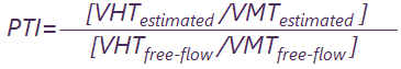 Figure 10. Equation. Planning Time Index.
Note: Both of the above measures of reliability are more appropriate for freeway-oriented corridor travel. For arterials and control-side targeted interventions, other measures from the travel time distribution may be preferable. In particular, extracting the standard deviation of the travel time distribution along paths or subpaths would be more meaningful in this project.
The report recommends assessing ATDM strategies for peak hours (same as HCM) but over all of the weekdays rather than a single weekday (different from HCM). In most available network models, demand data are not available for an entire week, but rather for representative operational conditions.
ANALYSIS, MODELING, AND SIMULATION TESTBED PERFORMANCE MEASURES
The following performance measures were considered candidates for collection during the Task 6 simulation experiments.
For all strategies: Standard deviation of the travel time distribution along paths or subpaths.
For adaptive signal control strategies:
- Stopped Time along links and subpaths.
- Travel Time along links and subpaths.
For reversible lanes:
- Corridor Speed.
- Corridor Travel Time.
Additional performance indicators specifically address travel time reliability. Figure 11 presents a list of available reliability measures, categorized on the basis of their applicability to different levels of travel time distributions and associated reliability analysis, namely network-level, ODlevel, and path/segment/link-level. For the network-level, travel times experienced by vehicles are not directly comparable because distances traveled by vehicles may be significantly different. In this case, measures that are normalized by the trip distance can be used. Each vehicle's travel time can be converted into the distance-normalized travel time, i.e., travel time per mile (TTPM) and various statistics can be extracted from the distribution of TTPMs as presented in Type A measures in Figure 11. For the OD-level, travel times experienced by vehicles are comparable, although actual trip distances could be different depending on the route followed by each vehicle. OD-level travel times are not limited to travel times between actual traffic analysis zones (TAZ). Travel time distributions between any two points can be included in this category. Reliability measures that can be used when travel times are comparable include many conventional metrics such as the mean and standard deviation of travel times, percentiles, buffer index, etc., as presented in Type B in Figure 11. For OD-level analysis, therefore, both Type A and B measures can be used. At the path/segment/ link-level, not only are travel times for different vehicles comparable but also trip distances are the same. This allows the calculation of unique free-flow travel times for a given path and, therefore, and allows the use of additional measures that require the free-flow travel time. Such measures include Travel Time Index, Planning Time Index, Misery Index and Frequency of Congestion as shown in Type C in Figure 11. As such, any Type A, B and C measures for the path/segment/linklevel can be used for travel time reliability analysis. For arterial analysis, Types B and C measures would be applicable measures for the path/segment/link-level travel time reliability analysis. For arterial analysis, Type B and C measures would be applicable.
Figure 11. Chart. Reliability measures for different analysis types
|
Analysis Level |
| Network-level |
00-level |
Path/Segment/Link-level |
| Distance-normalized Measures (Type A) |
- Average of TTPMs (Travel Time Per Mile)
- Std. Dev. of TTPMs
- 95th/90th/80th Percentile TTPM
|
- Average of TTPMs (Travel Time Per Mile)
- Std. Dev. of TTPMs
- 95th/90th/80th Percentile TTPM
|
- Average of TTPMs (Travel Time Per Mile)
- Std. Dev. of TTPMs
- 95th/90th/80th Percentile TTPM
|
| Measures for comparable travel times (Type B) |
|
- Average Travel Time
- Std. Dev of Travel times
- Coefficient of Variation
std. dev. of travel times/mean travel time
- 95th/90th/80th Percentile Travel Time
- Buffer Index
(95th percentile travel time-mean travel time/mean travel time)
- Skew Index
(95th percentile travel time-median travel time)/median travel time - 10th percentile travel time)
- Percentile On-time Arrival
percent of travel times < 1.1* median travel time
|
| Measures for the same travel distance (Type C) |
|
|
- TTI (Travel time Index)
mean travel time/free flow travel time
- PTI (Planning Time Index)
95th percentile travel time/free flow travel time
- Misery Index
mean of the highest 5% of travel times/ free flow travel time
- Frequency of Congestion
percent of travel times˃2* free-flow travel time
|
PERFORMANCE MEASURES FROM HIGHWAY CAPACITY MANUAL-BASED COMPUTATIONAL ENGINES
HCM-based computational engines could further assess the models developed by this project. The available HCM-based computational engines for urban streets are believed to be Streetval-Java (from the Institute for Transportation Research and Education (ITRE) at North Carolina State University) and HCS-Streets (from McTrans at the University of Florida). These two platforms have the necessary architecture needed for executing HCM-compliant annual reliability analyses, and generating advanced performance measures. The availability of these platforms for modification during this project's period of performance, and the effort level for incorporating this project's models into these platforms, was uncertain. However, the developers of both platforms expressed a willingness to assist on the urban streets ATDM project. Streetval-Java and HCS-Streets have different advantages, disadvantages, and sample datasets, which may affect the choice of platform (if any) to be used on this project. Streetval-Java is described first. Figure 12 illustrates a screenshot of reliability performance measures reported by Streetval. Currently, this screen shows travel time index (TTI)-related performance measure statistics at the bottom of the screen. The Streetval software also reports travel time, travel speed, stop rate, running time, through delay and total delay.
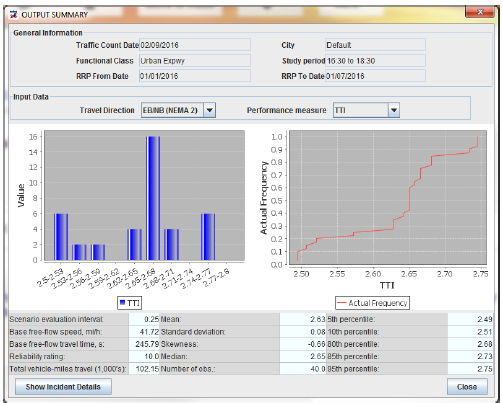 Figure 12. Screenshot. Performance measures available from Streetval-Java.
Source: ITRE, NC State University.
Figure 12. Screenshot. Performance measures available from Streetval-Java.
Source: ITRE, NC State University.
According to McTrans' Urban Streets Reliability Users Guide (from the HCS-Streets software package), there are two reports available to the user: the formatted report and the text report. The formatted report provides an overview of the results in a table. There are four sections in the table: base dataset analysis, reliability input summary, reliability performance measure results, and travel time results for each replication. Base dataset analysis provides general information that can be found in the base dataset. Reliability input summary provides general information on the reliability analysis and the random seed summary. The random seed numbers displayed on this report are for the first replication. Random seed numbers for each replication can be found in the text report. The formatted report is illustrated in Figure 13 and Figure 14.
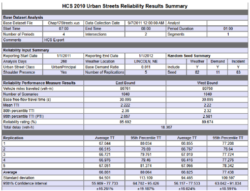 Figure 13. Screenshot. Reliability output summary report from HCS-Streets.
Source: McTrans Center, University of Florida
Figure 13. Screenshot. Reliability output summary report from HCS-Streets.
Source: McTrans Center, University of Florida
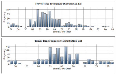 Figure 14. Chart. Travel time frequency from HCS-Streets.
Source: McTrans Center, University of Florida
Figure 14. Chart. Travel time frequency from HCS-Streets.
Source: McTrans Center, University of Florida
The formatted report section on "Reliability Performance Measure Results" provides information on the following performance measures for each major street direction: vehicle miles traveled (veh-m), number of scenarios, base free-flow travel time (s), mean TTI, 80th percentile TTI, 95th percentile TTI (PTI), reliability rating ( percent), and total delay (veh-h). The last section of the table includes information on travel time for each replication. The average travel time and 95th percentile travel time are provided in the formatted report. However the text report provides more detailed results, as shown in Figure 15.
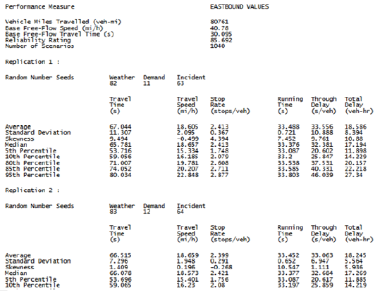 Figure 15. Screenshot. Detailed reliability outputs report from HCS-Streets
Source: McTrans Center, University of Florida
Figure 15. Screenshot. Detailed reliability outputs report from HCS-Streets
Source: McTrans Center, University of Florida
Results for the major street forward direction are displayed first, and then results for the other major street direction are displayed. The following performance measures are displayed for each major street direction: vehicle miles traveled (veh-mi), base free-flow speed (mi/h), base free-flow travel time (s), reliability rating, and number of scenarios. Following these results, information for each are replications. Each replication displays the random number of seeds for weather, demand, and incident. Then the average, standard deviation, skewness, median, 5th percentile, 10th percentile, 80th percentile, 85th percentile, and 95th percentile are displayed for travel time (s), travel speed (mi/h), stop rate (stops/veh), running time (s), through delay (s/veh), and total delay (veh-hr).
CONCLUSIONS AND NEXT STEPS
The dilemma revealed by this chapter is that desired reliability-based performance measures, such
as travel time index and planning time index, were generally not collected during the available field studies. Instead, the available field studies (whose results were summarized earlier in Figure 9) focused on travel times and delays. Thus, the only way to integrate these results with Task 6 simulation results would be to collect travel times and delays during Task 6. Having said this, the amount of available data for reversible/dynamic lanes was extremely limited, and the amount of available data for adaptive signals was insufficient for developing a reliable model. As such, the performance measures from available data sources (Task 4) would not be considered a constraint on the remainder of the project (Tasks 5 and 6), and project outcomes would be heavily dependent upon the original research in Task 6. Moreover, the HCM-compatible computational engines could provide an effective vehicle for obtaining most desired performance measures, if the urban street ATM methods could be successfully implemented within them.