Freight Analysis Framework Inter-Regional Commodity Flow Forecast Study
Final Forecast Results Report
PDF Version, 1.8 MB
You may need the Adobe® Reader® to view the PDFs on this page.
Contact Information: Operations Feedback at FreightFeedback@dot.gov

U.S. Department of Transportation
Federal Highway Administration
Office of Operations
1200 New Jersey Avenue, SE
Washington, DC 20590
FHWA-HOP-16-043
May 2016
Notice
This document is disseminated under the sponsorship of the U.S. Department of Transportation in the interest of information exchange. The U.S. Government assumes no liability for the use of the information contained in this document. This report does not constitute a standard, specification, or regulation.
The US Government does not endorse products or manufacturers. Trademarks or manufacturers' names appear in this report only because they are considered essential to the objective of the document.
Quality Assurance Statement
The Federal Highway Administration (FHWA) provides high-quality information to serve Government, industry, and the public in a manner that promotes public understanding. Standards and policies are used to ensure and maximize the quality, objectivity, utility, and integrity of its information. FHWA periodically reviews quality issues and adjusts its programs and processes to ensure continuous quality improvement.
Technical Report Documentation Page
| Form DOT F 1700.7 (8-72) Reproduction of completed page authorized | |||
|
1. Report No. FHWA-HOP-16-043 |
2. Government Accession No. | 3. Recipient's Catalog No. | |
|
4. Title and Subtitle Freight Analysis Framework Inter-Regional Commodity Flow Forecast Study: Final Forecast Results Report |
5. Report Date May 2016 |
||
| 6. Performing Organization Code | |||
|
7. Author(s) Richard Fullenbaum, Christopher Grillo |
8. Performing Organization Report No. | ||
|
9. Performing Organizations Name And Address IHS Global, Inc. 24 Hartwell Avenue Lexington, Massachusetts 02421 |
10. Work Unit No. (TRAIS) | ||
|
11. Contract or Grant No. DTFH61-11-D-00011/5002 |
|||
|
12. Sponsoring Agency Name and Address Federal Highway Administration Office of Freight Management and Operations 1200 New Jersey Ave SE Washington, DC 20590 |
13. Type of Report and Period Covered Technical Report (August 2015 - May 2016) |
||
|
14. Sponsoring Agency Code HOP |
|||
| 15. Supplementary Notes | |||
|
16. Abstract This technical report accompanies the 2012 base-year Freight Analysis Framework Forecasts (FAF4) submitted to the FHWA Office of Freight Management and Operations. The technical report outlines the data and methodology employed to develop freight forecasts using the 2012 base-year FAF data for 2013, 2014, 2015, 2016, and long-term forecasts in five-year increments from 2020 to 2045. This report also analyzes the resulting FAF4 forecasts, summarizing the observed trends and the outlook for domestic, imported, and exported goods movement for the United States. Included are detailed breakdowns by major commodity class and, for international trade, by key trade region. Three scenarios driven by different macroeconomic assumptions are analyzed and presented. |
|||
|
17. Key Words FAF, Freight Flows, Commodity Flows, Inter-regional Freight, Goods Movement, Multimodal Transportation, Intermodal Transportation |
18. Distribution Statement No restrictions |
||
| 19. Security Classif. (of this report) | 20. Security Classif. (of this page) |
21. No. of Pages 80 |
22. Price |
SI* (MODERN METRIC) CONVERSION FACTORS
| SYMBOL | WHEN YOU KNOW | MULTIPLY BY | TO FIND | SYMBOL |
|---|---|---|---|---|
| LENGTH | ||||
| in | inches | 25.4 | millimeters | mm |
| ft | feet | 0.305 | meters | m |
| yd | yards | 0.914 | meters | m |
| mi | miles | 1.61 | kilometers | km |
| AREA | ||||
| in2 | square inches | 645.2 | square millimeters | mm2 |
| ft2 | square feet | 0.093 | square meters | m2 |
| yd2 | square yard | 0.836 | square meters | m2 |
| ac | acres | 0.405 | hectares | ha |
| mi2 | square miles | 2.59 | square kilometers | km2 |
| VOLUME | ||||
| fl oz | fluid ounces | 29.57 | milliliters | mL |
| gal | gallons | 3.785 | liters | L |
| ft3 | cubic feet | 0.028 | cubic meters | m3 |
| yd3 | cubic yards | 0.765 | cubic meters | m3 |
| NOTE: volumes greater than 1000 L shall be shown in m3 | ||||
| MASS | ||||
| oz | ounces | 28.35 | grams | g |
| lb | pounds | 0.454 | kilograms | kg |
| T | short tons (2000 lb) | 0.907 | megagrams (or "metric ton") | Mg (or "t") |
| TEMPERATURE (exact degrees) | ||||
| F | Fahrenheit | 5 (F-32)/9 or (F-32)/1.8 |
Celsius | oC |
| ILLUMINATION | ||||
| fc | foot-candles | 10.76 | lux | lx |
| fl | foot-Lamberts | 3.426 | candela/m2 | cd/m2 |
| FORCE and PRESSURE or STRESS | ||||
| lbf | poundforce | 4.45 | newtons | N |
| lbf/in2 | poundforce per square inch | 6.89 | kilopascals | kPa |
| SYMBOL | WHEN YOU KNOW | MULTIPLY BY | TO FIND | SYMBOL |
|---|---|---|---|---|
| LENGTH | ||||
| mm | millimeters | 0.039 | inches | in |
| m | meters | 3.28 | feet | ft |
| m | meters | 1.09 | yards | yd |
| km | kilometers | 0.621 | miles | mi |
| AREA | ||||
| mm2 | square millimeters | 0.0016 | square inches | in2 |
| m2 | square meters | 10.764 | square feet | ft2 |
| m2 | square meters | 1.195 | square yards | yd2 |
| ha | hectares | 2.47 | acres | ac |
| km2 | square kilometers | 0.386 | square miles | mi2 |
| VOLUME | ||||
| mL | milliliters | 0.034 | fluid ounces | fl oz |
| L | liters | 0.264 | gallons | gal |
| m3 | cubic meters | 35.314 | cubic feet | ft3 |
| m3 | cubic meters | 1.307 | cubic yards | yd3 |
| MASS | ||||
| g | grams | 0.035 | ounces | oz |
| kg | kilograms | 2.202 | pounds | lb |
| Mg (or "t") | megagrams (or "metric ton") | 1.103 | short tons (2000 lb) | T |
| TEMPERATURE (exact degrees) | ||||
| oC | Celsius | 1.8C+32 | Fahrenheit | oF |
| ILLUMINATION | ||||
| lx | lux | 0.0929 | foot-candles | fc |
| cd/m2 | candela/m2 | 0.2919 | foot-Lamberts | fl |
| FORCE and PRESSURE or STRESS | ||||
| N | newtons | 0.225 | poundforce | lbf |
| kPa | kilopascals | 0.145 | poundforce per square inch | lbf/in2 |
Table of Contents
- Introduction
- Key Assumptions
- Forecast Results
- Forecast Methodology
- Underlying Forecast Drivers: Data Sources
- Appendix
List of Figures
- Figure 1. Graph. Compound Annual Growth Rates for Domestic, Import, and Export Tonnage Forecasts for Selected Time Periods
- Figure 2. Graph. Total Domestic Freight Flows, 2012 — 2045
- Figure 3. Graph. Compound Annual Growth Rates (2012 — 2045) by Commodity and Tonnage
- Figure 4. Graph. Total Real Values of Domestic Freight Flows, 2012 — 2045
- Figure 5. Graph. Total Export Flows, 2012 — 2045
- Figure 6. Graph. U.S. Exports by Destination Region, 2012 — 2045
- Figure 7. Graph. Real Values of Total Export Freight Flows, 2012 — 2045
- Figure 8. Graph. Total Import Freight Flows, 2012 — 2045
- Figure 9. Graph. U.S. Imports by Region of Origin, 2012 — 2045
- Figure 10. Graph. Real Value of Import Freight Flows, 2012 — 2045
- Figure 11. Graph Domestic Tonnages — Baseline, Optimistic, and Pessimistic Scenarios, 2015 — 2045
- Figure 12. Graph. Domestic Optimistic and Pessimistic Scenario Variations from the Baseline Scenario, 2015 — 2045
- Figure 13. Graph. Export Tonnages — Baseline, Optimistic, and Pessimistic Scenarios, 2015 — 2045
- Figure 14. Graph. Import Tonnages — Baseline, Optimistic, and Pessimistic Scenarios, 2015 — 2045
- Figure 15. Graph. Variations in Import and Export Tonnage from Baseline, Optimistic, and Pessimistic Scenarios, 2015 — 2045
- Figure 16. Chart. Overview of the IHS Model of the U.S. Economy
List of Tables
- Table 1. U.S. Macroeconomic Forecast Historical and Forecasted Indicators to 2020
- Table 2. Long-Term U.S. Macroeconomic Forecasted Indicators to 2045
- Table 3. U.S. Macroeconomic Snapshot — January 2016
- Table 4. Top Five Domestic Commodity Classes, 2012 and 2045
- Table 5. U.S. Exports by Destination Region, 2012 and 2045
- Table 6. U.S. Imports by Region of Origin, 2012 and 2045
- Table 7. Growth in Domestic Tonnage under Baseline, Optimistic, and Pessimistic Scenarios, 2012 — 2045
- Table 8. Growth in Exported Tonnage under Baseline, Optimistic, and Pessimistic Scenarios, 2012 — 2045
- Table 9. Growth in Imported Tonnage under Baseline, Optimistic, and Pessimistic Scenarios, 2012 — 2045
- Table 10. WTS Import/Export Drivers by Standard Classification for Transported Goods Code
1 Introduction
The United States (U.S.) Department of Transportation (DOT) Federal Highway Administration (FHWA) administers the Freight Analysis Framework (FAF) to periodically survey goods movement to, from, and within the US, and to use that data to develop long-term forecasts for commodity flows between domestic and international origin-destination pairs. The FHWA, with the help of the Bureau of Transportation Statistics (BTS), develops detailed base-year freight flow data every five years through the Commodity Flow Survey (CFS). The most up-to-date data was released in early 2016, with 2012 as the base year. The FHWA then works with public and private entities to apply macroeconomic data and industry research in order to forecast this base-year data as inter-regional freight flows, domestic and international, through 2045.
The Final Forecast Results Report describes the assumptions, methodology and approach, and final results in the development of the 2012 base-year Freight Analysis Framework Inter-Regional Commodity Flow Forecast Study. For brevity, the study and forecasts will be referred to throughout this document as "FAF4", as this version represents the fourth generation of FAF1. The report covers forecasts derived from Version 4.1 or the FAF4 base-year database (FAF4.1). The forecasts are developed using data and assumptions provided by third-parties which, by themselves, do not necessarily represent the views of the FHWA or the U.S. Federal Government.
In keeping with the structure of the FAF4 base-year database, the FAF4 Forecasts are provided for 132 mutually-exclusive regions that fully partition the 50 States and the District of Columbia. Moreover, exports from and imports to these 132 regions are forecasted with respect to 8 international regions. The flow forecasts are further disaggregated by 7 domestic and 8 international modes of transportation and by 43 domestic and 42 international commodity classes. The result is a detailed database of forecasted domestic and international freight flows into and out of each CFS-defined region2.
This document is organized into four major sections. The Key Assumptions section summarizes the macroeconomic trends and factors affecting U.S. domestic and international commodity flows. The Forecast Results section summarizes the resulting FAF4 Final Forecasts for the Baseline, Optimistic, and Pessimistic scenarios. The Forecast Methodology section describes the processes by which macroeconomic and industry forecasts are applied to the FAF4 2012 base-year data set to produce the FAF4 Forecasts. The Underlying Forecast Drivers: Data Sources section then describes in greater detail the primary products and services used to develop the macroeconomic drivers of the FAF4 Forecasts.
2 Key Assumptions
This section of the report describes the key macroeconomic assumptions underpinning the Freight Analysis Framework (FAF) Fourth Generation (FAF4) Forecasts. As a preface to the overview of the FAF4 Forecasts, it is important to review the assumptions that drive the long-term economic forecasts because they directly influence the results. The Forecast Methodology section of this document later describes in detail the processes by which the long-term macroeconomics assumptions are combined with the FAF 2012 base-year database, resulting in the FAF4 Forecasts.
The FAF4 Forecasts are driven by the most up-to-date macroeconomic assumptions on the short- and long-term trends of the United States (U.S.) economy at the time of the FAF4 Forecasts development (January 2016) as the basis for inter-regional domestic and international freight flows tonnage and value forecasts. These assumptions about the national economy form the basis of national-level forecasts of output, consumption, and trade, by industry for the various FAF regions, which are ultimately applied to the FAF4 base-year database to drive the FAF4 Forecasts.
Because the macroeconomic assumptions are provided by a third-party, the views summarized in this section do not necessarily reflect the views of the Federal Highway Administration (FHWA) or the Federal Government. Rather, the data and models derived from these assumptions are procured to enhance Government-published data. The FAF4 base-year database is compiled and published by the FHWA, using information collected from freight transportation operators as part of the most recent five-year Commodity Flow Survey (CFS) and from other information sources. The process of combining third-party and Federal Government data results in forecasts for years 2013, 2014, 2015, and 2016 and long-term forecasts in five-year increments from 2020 to 2045.
This section describes a baseline macroeconomic scenario for the U.S. economy, as well as two alternative cases. These scenarios guide the development of various macroeconomics and industry forecasting data applied in this study. These macroeconomic inputs drive, respectively, the Baseline, Optimistic, and Pessimistic FAF4 Forecasts summarized in this FAF4 Final Forecast Results Report.
2.1 Baseline U.S. Economy Outlook3
The IHS January 2016 U.S. Economy Macroeconomic Outlook suggests that the U.S. economic fundamentals remain solid, despite weak top-line growth in the third and fourth quarters of 2015. The Outlook, which summarizes U.S. macroeconomic forecasts to 2020, highlights the following recent and expected future trends:
- Real Gross Domestic Product (GDP) growth in the third quarter of 2015 (2.0 percent) was about half the rate of second-quarter growth (3.9 percent).
- Almost all of the slower growth can be attributed to an (expected) inventory correction. Real final sales by domestic purchasers, GDP less inventories and exports, grew by 2.9 percent.
- Household spending growth remained robust, with real consumer expenditures up 3.0 percent in the third quarter of 2015, and residential investment increased 8.2 percent. Estimates suggest slightly lower growth in consumer expenditures (2.4 percent) and residential investment (6.3 percent) in the fourth quarter of 2015.
- In an indication of strong fundamentals, real final sales of domestic product (GDP less private inventory change) rose 3.0 percent in the third quarter of 2015.
- Real growth fell to 1.2 percent in the fourth quarter of 2015 but, with the inventory cycle beginning to ease, is expected to rebound to 3.0 percent in the first quarter of 2016.
- Calendar-year growth is forecasted to rise from 2.4 percent in 2015 to 2.7 percent in 2016.
- In another sign of strength, after two weak months, the job market showed strength in December of 2015, with gains of 292,000. This brings the three-month average to 284,000.
- The $1.1 trillion omnibus spending bill and the reauthorization of Federal transportation programs will have a small but positive impact on growth in 2016, while also significantly reducing policy uncertainty.
- The Federal Reserve elected to increase the Federal Funds Rate in December of 2015. The Federal Reserve based this decision on its analysis of intervening data, particularly the improved employment situation.
The slower GDP growth experienced in the second half of Calendar Year 2015, which fell from an annualized 3.9 percent in the second quarter to 2.0 percent in the third quarter and 1.2 percent (estimated) in the fourth quarter, is attributable to three negative influences: the strong dollar, the collapse in oil sector investment, and the recent inventory cycle. The worst of the oil sector's capital spending drop is over and the inventory correction is winding down, meanwhile lower energy costs are helping U.S. manufacturers facing headwinds on exports due to the strong dollar. Therefore, some of the headwinds contributing to the recent deceleration of growth appear to be subsiding.
At the same time, there are a number of positive signs for U.S. economic growth. Robust service-sector growth and employment growth (unemployment has fallen to 5 percent) combined with lower gasoline prices, decreasing consumer debt, and increasing incomes and real wages will continue to boost consumer confidence and spending. While some sectors such as business fixed investment and construction slowed in the second half of 2015, this is partly due to rebalancing after extraordinarily high growth in these sectors in the first half of the year. These sectors will accelerate again in 2016, with strong November housing starts data already pointing towards improved construction sector growth. A return of modest growth in government spending (especially State and local government spending and transportation spending resulting from the reauthorization of Federal transportation programs) and government employment combined with Federal budgetary policy and continued low Federal Government interest rates will help support an acceleration of growth to 2.7 percent in 2016.
In the medium term, U.S. GDP growth will accelerate, peaking in 2017 at 2.9 percent and tapering off slightly by 2020 to 2.4 percent. The key assumptions include a return in oil and gas industry capital investment (whose decline has disproportionately affected growth in extraction regions of the US), a tightening of U.S. monetary policy, and the eventual appreciation of other currencies premised on continued strength in real disposable income growth, further growth in auto sales, increasing household real estate wealth, and modest consumer price inflation. Employment will continue to grow but at a slower relative pace, as companies try to strike a balance between adding payroll and increasing productivity.
In terms of trade, imports will outpace exports for the next two years, constraining growth. This is due to appreciation of the U.S. dollar as well as a likely increase in petroleum imports, as the recent shrinking of U.S. petroleum imports (in favor of domestic production) reaches a near-term natural limit. Export growth rates will begin to exceed import growth rates again beginning in 2018 when GDP in many foreign countries begins to grow, pulling up foreign currencies and making U.S. manufacturing more cost competitive.
The following table forecasted key macroeconomic drivers of the U.S. economy through 2020.
| 2012 | 2013 | 2014 | 2015 | 2016 | 2017 | 2018 | 2019 | 2020 | |
|---|---|---|---|---|---|---|---|---|---|
| Source: IHS | |||||||||
| Gross Domestic Product Growth (percent change) |
2.2 | 1.5 | 2.4 | 2.4 | 2.7 | 2.9 | 2.6 | 2.4 | 2.4 |
| Industrial Production (percent change) |
2.8 | 1.9 | 3.7 | 1.3 | 0.6 | 3.0 | 2.9 | 2.6 | 2.8 |
| Non-residential Fixed Investment (percent change) |
9.0 | 3.0 | 6.2 | 3.4 | 5.0 | 5.0 | 4.7 | 3.9 | 3.9 |
| Light Vehicle Sales (million units) |
14.44 | 15.53 | 16.44 | 17.39 | 17.76 | 18.19 | 18.07 | 17.70 | 17.28 |
| Housing Starts (million units) |
0.784 | 0.928 | 1.001 | 1.109 | 1.265 | 1.419 | 1.509 | 1.559 | 1.597 |
| Productivity (percent change) |
0.2 | 0.4 | 0.4 | 0.5 | 1.4 | 1.7 | 1.9 | 2.0 | 1.9 |
With regard to the long term, beyond 2020 it is assumed that the U.S. economy exists in an environment free of exogenous shocks. Economic output will converge towards its potential level, with all resources fully utilized. As a result, the growth rates of output, real incomes, real expenditures, and the general standard of living of the population are determined by the growth rate of potential GDP. The long-range outlook is dominated by supply factors, such as population growth and demographics, labor force participation rates, average weekly hours worked, national saving and capital stock accumulation, and productivity growth. The following table summarizes long-term assumptions about the U.S. economy.
| 2025 | 2030 | 2035 | 2040 | 2045 | |
|---|---|---|---|---|---|
| Source: IHS | |||||
| Gross Domestic Product Growth (percent change) |
2.1 | 2.2 | 2.2 | 2.1 | 2.1 |
| Industrial Production (percent change) |
1.8 | 1.9 | 1.9 | 1.8 | 1.6 |
| Non-residential Fixed Investment (percent change) |
3.3 | 2.5 | 2.8 | 2.7 | 2.5 |
| Light Vehicle Sales (million units) |
17.13 | 17.93 | 18.25 | 18.78 | 19.68 |
| Housing Starts (million units) |
1.569 | 1.515 | 1.510 | 1.499 | 1.544 |
| Productivity (percent change) |
1.8 | 1.8 | 1.8 | 1.7 | 1.7 |
Alternative scenarios have also been developed for the FAF4 Forecasts by applying optimistic and pessimistic scenarios for the U.S. economy. The following table summarizes some of the underlying assumptions of the baseline scenario described in the previous paragraphs as well as the optimistic and pessimistic scenarios driving the FAF4 Forecasts, focusing on early years in the forecasting process.
In long-term out years, growth assumption factors remain higher for the optimistic case and lower for the pessimistic case. The differences among long-term growth rates across the scenarios are; however, more narrow than in early year, and generally deviating less than 0.5 percent from the baseline. The IHS Outlook assigns a 65 percent probability that the baseline case will occur, 20 percent to pessimistic case, and 15 percent to the optimistic case.
| Baseline (65 percent) | Pessimistic (20 percent) | Optimistic (15 percent) | |
|---|---|---|---|
| Source: IHS | |||
| Gross Domestic Product Growth | Moderate growth, 2.7 percent in 2016 and 2.9 percent in 2017 | Growth slumps to 0.9 percent in 2016 with a recession in the second and third quarters | Stronger rebound as improved wages and payroll employment feed a housing recovery, up 3.4 percent in 2016 and 3.9 percent in 2017 |
| Consumer Spending | Moderately strong, up 3.0 percent in 2016 and 3.2 percent in 2017 | Slows sharply, up 1.9 percent in each of 2016 and 2017 | Economy leader as incomes rise, up 2.9 percent in 2016 and 3.9 percent in 2017 |
| Business Fixed Investment | Solid, up 5.0 percent in 2016 and 2017 | Stalls, up 1.8 percent in 2016 and 0.7 percent in 2017 | Stronger, up 6.0 percent in 2016 and 7.4 percent in 2017 |
| Housing | Gradual improvement, with more than 1.3 million starts by the end of 2016 | Construction stagnates, and starts decline to 1.1 million in 2016 | Pace of building rises, with nearly 1.5 million starts by late 2016 |
| Exports | Modest, with 2.3 percent growth in 2016 and a 5.4 percent jump in 2017 | Strong dollar and global weakness damage exports, down 1.1 percent in 2016 and recovering to 2.8 percent in 2016 | Strong, up 5.4 percent in 2016 and 7.6 percent in 2017 |
| Fiscal Policy* | Bipartisan agreements fund existing obligations without interruption | Political paralysis prevents any meaningful fiscal action during the current and future administrations | Budget gap narrows as policymakers slow the pace of spending growth, while taking in more revenue |
| Monetary Policy* | The Federal Reserve hikes the Federal Funds Rate four times in 2016, ending the year at 1.5 percent | The Federal Reserve abstains from additional rate increases until 2018; thereafter, the funds rate remains elevated in the face of inflationary pressure | Interest rates rise above 2 percent in 2016 and settle just beneath the 4 percent range in the longer term |
| Credit Conditions* | Gradually easing | Lending standards remain high | Rapidly easing |
| Productivity Growth | Modest, averaging 1.6 percent during 2016—25 | Stagnates and fails to improve rapidly, averaging 1.2 percent during 2016—25 | Takes off in 2016, averaging 1.9 percent during 2016—25 |
| Consumer Confidence | Peaks in late 2016 and remains roughly stable | Plunges through mid-2017 and begins a slow recovery thereafter at depressed levels | Rebounds strongly through mid-2018 and then retreats, leveling off higher than in the baseline |
| Oil Prices (Dollars/barrel) | Brent crude oil price averages $48 in 2016 and $58 in 2017 | Brent crude oil price averages $43 during 2016 and rebounds to $57 in 2017, exceeding the baseline thereafter as supply tightens | Brent crude oil price rises to $64 by the end of 2016 but trends below the baseline thereafter |
| Stock Markets* | The S&P 500 maintains steady growth, averaging 3.0 percent in 2016 and 3.2 percent between 2017-25 | S&P 500 contracts sharply in mid-2016 on a wave of global weakness and equities are devalued, regaining early-2015 levels only by 2018 | The S&P 500 grows at a brisk pace of 6.8 percent in 2016 and averages 3.7 percent between 2017 and 2025 |
| Inflation (Consumer Price Index) | Headline Consumer Price Index inflation picks up in 2016 as lower oil prices begin to reverse; core inflation hits 1.9 percent in 2016 and 2.0 percent 2017 | Weak demand keeps inflation below 2.0 percent until 2017 but an inflationary environment takes hold and inflation exceeds the baseline starting in late 2017 | Core prices exceed the baseline through 2017 but then rejoin it in 2020 |
| Foreign Growth | In 2016, Eurozone growth will proceed around 1.7 percent and China’s will slow to 6.3 percent | Developing markets suffer a slowdown and Europe undergoes contraction; global growth stagnates | Global growth picks up, with developed economies and emerging markets experiencing strong accelerations |
| U.S. Dollar | The inflation-adjusted dollar appreciates 6.4 percent against the broad index of trading partners’ currencies in 2016 and begins declining in the third quarter | Appreciates faster than the baseline through early 2016, then depreciates at a faster pace thereafter | World-leading growth causes appreciation against other currencies from late 2016 through mid-2018 |
3 Forecast Results
This section summarizes the Freight Analysis Framework (FAF) Fourth Generation (FAF4) Forecasts. The content summarizes the Baseline Forecast and the relative growth trajectories of the Optimistic and Pessimistic forecasts for domestic, import, and export freight flows. In addition, imports and exports for historical forecast years (2013 and 2014) are calibrated to actual provisional data available through various Federal Government sources, where available. This ensures that 2013 and 2014 international tonnage and value flow forecasts match actual data, to the extent feasible.
The forecasts are driven by macroeconomic data derived from a national model for which FAF-zone-level data is fully integrated. In some cases modifications are applied to the inputs and processes for certain origin-destination-commodity combinations where the overarching methodology and process produces unrealistic growth rates. This is primarily due to situations where FAF-zone-level industry employment and/or output growth rates are poor indicators of traffic growth (e.g., the "headquarters effect") or where major shifts in production and consumption patterns are expected to occur. These issues and the subsequent adjustments are described in detail in the Forecast Methodology section.
3.1 Baseline Scenario
The FAF4 Forecasts Baseline Scenario has three parts: domestic, imports, and exports. The total tonnage compound average annual growth rate (CAGR) is 1.2 percent from 2012 to 2045. Growth will be highest through 2014, reflecting the United States (U.S.) economy's rebound from the Great Recession as well as manufacturing and exports growth during the historical forecast years of 2012-2014. Growth in tonnage will slow from 2015-2020 to 1.7 percent, reflecting the strong but modest economic growth forecasted for the short- and medium-term described in Section 2 of this report.
Over the final 25 years of the forecast period, freight growth rates moderate further to 1.0 percent, reflecting a longer-term structural analysis of the U.S. economy. Between 2020 and 2045, imports and especially exports grow more rapidly, at 2.5 percent and 2.7 percent, respectively. However, domestic flows fall to 0.8 percent, partially reflecting lower long-term growth in U.S. domestic output as well as changing energy consumption patterns. Total tonnage increases from 17.0 billion tons in 2012 to 25.3 billion tons in 2045.
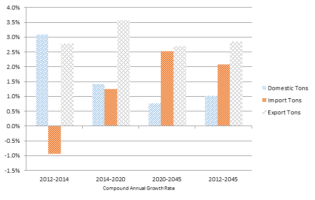
Figure 1. Graph. Compound Annual Growth Rates for Domestic, Import, and Export Tonnage Forecasts for Selected Time Periods
3.1.1 Domestic Freight Flows
In the Baseline Scenario, total domestic freight flow tonnage grows by 6.0 billion tons over the forecast period of 2012 to 2045, an increase of just over 40 percent, or a 1.0 percent CAGR. However, that 33-year view masks some key short-term trends. Specifically, the early years of the forecast period exhibit much higher growth due to recovery from the nadir of the Great Recession. Moreover it reflects a generally stronger outlook earlier in the forecast period, as recent trends favor more modest but historically robust growth from 2014-2020 of about 1.4 percent. This more modest but still relatively strong growth in domestic tonnage reflects the mostly favorable, albeit diminishing, macroeconomic tailwinds through 2020, as described in Section 2 of this report. After 2020, the rate of growth is expected to slow to a steady 0.8 percent CAGR partially reflecting a lower overall U.S. economic growth potential. However, another major factor weighing down long-term growth rates is the changing pattern of energy consumption and production in the US, which will be described in greater detail later in this sub-section.
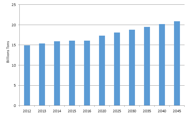
Figure 2. Graph. Total Domestic Freight Flows, 2012 — 2045
The five Standard Classification of Transported Goods (SCTG) classes with the highest domestic traffic in the FAF4 base-year database are Coal and Petroleum Products (SCTG 19, including natural gas, natural gas liquids, petroleum coke, and related commodities), Gravel and Crushed Stone (12), Gasoline (17), Coal (15), and Nonmetallic Mineral Products (31). These five commodity classes represent about 46 percent of the total purely domestic tonnage moved in 2012. By 2045, however, several major shifts occur. Most notably, coal continues its significant decline, falling to 12th in the rankings. This reflects the continued shift in U.S. domestic power generation to natural gas (driving SCTG 19; still the largest domestic commodity class in 2045) and, to a lesser extent, renewables. Gravel and Crushed Stone remains the second largest domestic commodity class, averaging 1.0 percent growth from 2012 to 2045. This is the result of new construction and ongoing maintenance and repair of an aging U.S. infrastructure network, all of which is linked in part to economic growth.
Cereal Grains (SCTG 02) and Other Foodstuffs (SCTG 07) enter the top five rankings by 2045. Growth in Cereal Grains generally reflects the expected long-term growth in production and consumption of food in the US, and is a rough proxy for population growth in an advanced economy. The Other Foodstuffs commodity class growth suggests increased demand for manufactured food products, reflecting population and income growth. Adding domestic Cereal Grains and Other Foodstuffs flows to the 2012 top five domestic commodity classes represents 56 percent of the total tonnage in the base year.
| Standard Classification for Transported Goods Class and Number | Tonnage and Rank, 2012 | Tonnage and Rank, 2045 | Compound Annual Growth Rate, 2012-2045 |
|---|---|---|---|
| Coal and Petroleum Products (19) | 2.22 billion tons, 1 | 3.89 billion tons, 1 | 1.7 percent |
| Gravel and Crushed Stone (12) | 1.74 billion tons, 2 | 2.43 billion tons, 2 | 1.0 percent |
| Gasoline (17) | 1.04 billion tons, 3 | 961 million tons, 6 | -0.2 percent |
| Coal (15) | 997 million tons, 4 | 540 million tons, 12 | -1.8 percent |
| Nonmetallic Mineral Products (31) | 920 million tons, 5 | 1.60 billion tons, 3 | 1.7 percent |
| Cereal Grains (02) | 871 million tons, 6 | 1.21 billion tons, 4 | 1.0 percent |
| Other Foodstuffs (07) | 620 million tons, 8 | 1.04 billion tons, 5 | 1.6 percent |
Several declining commodity classes are related to the energy sector. Nuance is important in interpreting these results. In addition to general macroeconomic conditions, industry-specific factors contribute significantly to the forecasts. First, coal, which is primarily used for the generation of electricity, is in a structural decline as represented by an average forecasted decline of 1.8 percent over the forecast period. The discovery and economic extraction of domestic natural gas combined with lower capital costs for new gas-fired power plants is significantly altering the long-term U.S. energy consumption profile. Development of renewable-powered generation and compliance with environmental regulations will also contribute to declining shares of coal-fired power generation. Meanwhile, the growth in domestic energy products used primarily for motor vehicle fuel such as gasoline and diesel (the former is a component of SCTG 17, while the latter is a component of SCTG 18) peaks around 2020 as fuel efficiency standards and changing transportation patterns drive 2045 consumption below 2012 levels.
Domestic Crude Petroleum (SCTG 16) flows grow throughout most of the forecast period, before falling below base-year 2012 levels by 2045. Despite declining domestic growth for gasoline and diesel beginning in the 2020s, U.S. refineries will increase consumption of low-cost, domestically produced crude petroleum. The increased production of petroleum products at U.S. refineries will be reflected strongly in SCTG 17 and SCTG 18 export growth. This dynamic will be described in the exports forecast summary following this sub-section. Nonetheless, the forecasted peaking of domestic unconventional shale oil plays will contribute to long-term declines in domestic crude oil production and domestic refinery consumption.
While most domestic energy SCTG classes decline over the long term, one grows rapidly. Two of the larger components of the Coal and Petroleum Products class are natural gas and natural gas liquids. The SCTG 19 flows are forecasted to rise through 2045 by 1.7 percent, compounded annually. As previously described, natural gas will displace coal demand for domestic power generation, while natural gas liquids will supply a rejuvenated chemicals manufacturing base. The impact on domestic chemicals, especially Fertilizers (SCTG 22) and Plastics and Rubber (SCTG 24), will be described later in this sub-section. It is important to note that natural gas and natural gas liquids will probably grow by more than 1.7 percent; however, the overall SCTG 19 growth rate will be weighed down by slowing domestic petroleum coke consumption.
It is also important to note that there is uncertainty in the magnitude in shifts of long-term trade and supply chains resulting from the growth of U.S. unconventional energy extraction. The industry forecasts used in this study for energy-related products are roughly consistent with U.S. Energy Information Administration (EIA) forecasts for SCTGs 16-18. The forecasts differ somewhat for SCTG 15 and SCTG 19; however, as the data sources employed in this study assume a more rapid decline in coal consumptions and a more rapid increase in natural gas consumption for domestic power generation.
Figure 3 plots 2012 tonnage to CAGRs over the forecast interval. The chart shows that the fastest growing domestically moved commodities over the forecast interval also generally make up some of the smaller commodity groups tonnage-wise. The clustering in the upper left hand corner illustrates the trend in high growth rates for small-tonnage, high-value commodities.
This growth in small-tonnage, high-value commodities illustrates the transition of the U.S. manufacturing base towards producing lighter, higher-value goods requiring more technically advanced processes. The fastest growing commodity groups from 2012-2045, Pharmaceuticals (SCGT 21, 2.8 percent), Precision Instruments (SCTG 38, 2.7 percent), and Transport Equipment (SCTG 37, 2.7 percent), are among the five smallest commodity classes in terms of tonnage. Electronics (SCTG 35) is larger in terms of tonnage and includes many now-commoditized products (that is, products that are not differentiable by quality or producer but are largely homogeneous), but this advanced technology class still registers a 2.5 percent CAGR.
Figure 3 also illustrates several outliers. Tobacco Products (SCTG 09) flows decline rapidly due to changing U.S. consumption patterns. Meanwhile, Textiles and Leather (SCTG 30) declines due to trends towards imports of apparel. High-tonnage Gravel and Crushed Stone grows with increased construction demand, especially for infrastructure maintenance. Meanwhile, the chart captures the aforementioned displacement of Coal by Coal and Petroleum Products (i.e., natural gas), and the growth of natural gas liquids.
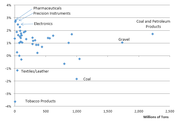
Figure 3. Graph. Compound Annual Growth Rates (2012 — 2045) by Commodity and Tonnage
The "re-shoring" of automotive manufacturing in the US, both in the Great Lakes region but especially in the Southeast, has been driving up domestic production for the U.S. market in recent years. This is reflected in the Motorized Vehicles (SCTG 36) domestic commodity flow growth rates, averaging about 5.3 percent compounded annually from 2012 to 2015. While domestic production and consumption of Motorized Vehicles should remain positive in the future, the high-growth phase has likely peaked. Positive but lower growth rates are forecasted in the future.
The forecasts suggest some mid-sized commodity groups among the fastest growing, especially in chemicals-related industries. Specifically, Fertilizers (1.3 percent, 19th largest commodity group by tonnage in 2012), Plastics and Rubber (1.9 percent, 20th), and Chemical Products (1.8 percent, 26th) register higher-than-average growth rates for domestic cargo flows from 2012 and 2045. Growth in these chemicals-related commodity classes (as well as Pharmaceuticals) relates to the resurgence of chemicals manufacturing in the US. As detailed previously, abundant petrochemical feedstocks from domestic unconventional oil and gas extraction has contributed to the massive current and planned expansion of chemicals manufacturing in the US. These new plants are concentrated on the U.S. Gulf Coast, but there may also be investment in states in the Marcellus and Utica shale play areas of the Appalachian Mountains (mainly Pennsylvania and West Virginia, but also possibly in Ohio, Kentucky, and New York). The US will switch from being a major importer to being a major exporter of numerous widely-traded petrochemical commodities, such as methanol.
The trend in real value of domestic freight follows the trend of tonnage growth. The following figure illustrates the growth in domestic commodity flow values, in real terms. The real value measure excludes the impact of inflation. From 2012 to 2014, real value grows by about $694 million (2.4 percent CAGR) from $14.1 trillion to $14.8 trillion, and then grows by another $1.7 trillion to $16.4 trillion by 2020 (1.8 percent CAGR). Over the entire period of this forecast, value grows from $14.1 trillion in 2012 to $22.5 trillion in 2045, representing a CAGR of 1.4 percent.
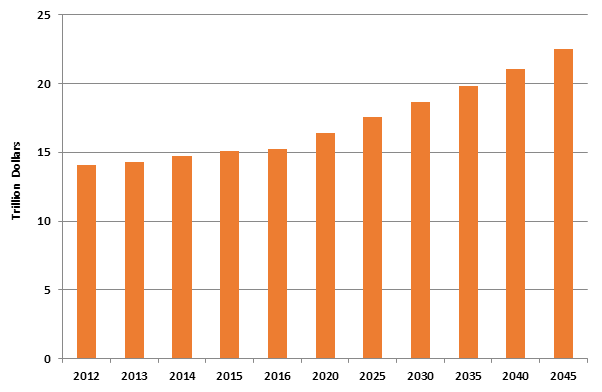
Figure 4. Graph. Total Real Values of Domestic Freight Flows, 2012 — 2045
According to this forecast, the growth rate of domestic freight real value (1.4 percent CAGR) exceeds the growth rate of tonnage (1.0 percent CAGR), indicating that the mix of domestically moved tonnage evolves over time toward higher-value commodities.
3.1.2 Export Freight Flows
In general, demand for U.S. exports is influenced by the relative values of the currency of the US and its trading partners, as well as the levels of demand for U.S.-produced goods from each trading partner. Since at least the Great Recession, a weak U.S. dollar has supported export growth generally in balance with, or greater than, imports. A weak dollar effectively makes goods produced in the US relatively cheaper for foreign consumers to buy. In addition, certain regions of the world weathered the recession of 2007-2009 better than others, particularly in developing economies, thus their demand growth for imports did not diminish as much as in the US.
The recent strengthening of U.S. growth compared to slower growth in Europe and many developing economies, combined with other factors such as monetary policy, has led to an appreciation of the U.S. dollar relative to other global currencies. This, in turn, will push import growth above export grown in the short term. The macroeconomic forecasts described in Section 2 suggest that this trend will persist until about 2018, when economic growth outside of the US accelerates, the dollar depreciates, and U.S. exports again rise faster than imports.
With exchange rates as the driving force, U.S. export tonnage is forecasted to grow at 2.8 percent from 2012-2014, as well as by about 2.9 percent over the entire forecast period. The following figure illustrates the export flow forecasts over the FAF4 Forecast period.
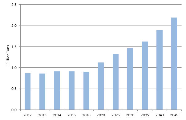
Figure 5. Graph. Total Export Flows, 2012 — 2045
Eastern Asia is the leading destination for U.S. exports, and trade will grow rapidly along this lane over the forecast period (3.6 percent CAGR). The region includes major trading partners: China, Japan, and South Korea. Greater integration, possibly through enhanced free-trade deals, as well as the continued growth in China and other major Eastern Asia consumer economies will help buttress this long-term trend.
The next two largest destinations are North American Free Trade Agreement (NAFTA) trade partners, Canada and Mexico. Canada is and will remain the second largest recipient of U.S. exports, growing at 2.6 percent compounded annually over the forecast period. Mexico will overtake Europe as the fourth largest destination, growing at 2.9 percent compounded annually over the forecast period. These growth rates reflect a general trend in cross-border trade between the US, Canada, and Mexico, and greater integration of the major North American economies.
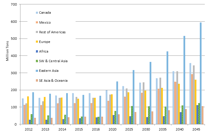
Figure 6. Graph. U.S. Exports by Destination Region, 2012 — 2045
Export growth to other regions will vary from 1.4 percent to 4.5 percent. Trade to Europe, currently the second largest recipient of U.S. exports, will grow the slowest to 2045. Headwinds on long-term economic growth in Europe result in lower consumer demand and, hence, lower demand for U.S. exports. Meanwhile, growth in Africa economies will propel compound annual growth in U.S. exports to the region by 4.5 percent through 2045.
| Region Code | Destination Region | Export Tons, 2012, millions | Export Tons, 2045, millions | Compound Annual Growth Rate, 2012-2045 |
|---|---|---|---|---|
| 801 | Canada | 151 | 357 | 2.6 percent |
| 802 | Mexico | 114 | 293 | 2.9 percent |
| 803 | Rest of Americas | 123 | 344 | 3.2 percent |
| 804 | Europe | 163 | 260 | 1.4 percent |
| 805 | Africa | 26 | 113 | 4.5 percent |
| 806 | SW & Central Asia | 60 | 123 | 2.2 percent |
| 807 | Eastern Asia | 188 | 595 | 3.6 percent |
| 808 | SE Asia & Oceania | 39 | 105 | 3.1 percent |
| Total | 864 | 2,190 | 2.9 percent |
As in the case of domestic freight flow forecasts, the real value of U.S. exports will outpace tonnage growth. The following table illustrates export value growth from $1.5 trillion in 2012 to $6.5 trillion by 2045, a CAGR of 4.1 percent, as compared to a 2.9 percent CAGR in tonnage.
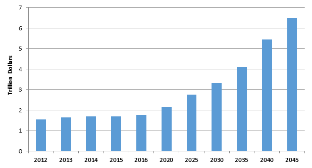
Figure 7. Graph. Real Values of Total Export Freight Flows, 2012 — 2045
3.1.3 Import Freight Flows
Demand for imports is also affected by the relative strength of the dollar versus other currencies, plus the overall U.S. demand for commodities. However, a weak dollar lessens the demand for imports, as imports become more expensive relative to domestically produced goods. Therefore, the overall trend in imports diverges from that of exports. The relatively weak dollar helps explain why imports are forecasted to grow slower than exports between 2012 and 2014; imports are forecasted to decline by a 0.9 percent CAGR over this period, while exports grow at a 2.8 percent CAGR. This trend is also partially a function of import substitution of petroleum products. Imports then grow rapidly with an appreciating dollar between 2014 and 2018, before a diminishing growth rate takes hold, relative to exports. The following figure illustrates the trends in U.S. import growth from 1.1 billion tons in 2012 to 2.2 billion tons in 2045 (2.1 percent CAGR).
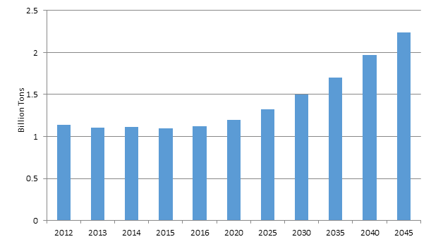
Figure 8. Graph. Total Import Freight Flows, 2012 — 2045
Canada and Mexico are, again, major trading partners for the US, with Canada being the largest origin for U.S. imports. Imports from Mexico; however, are growing faster (a 2.6 percent CAGR from Mexico versus a 2.2 percent CAGR from Canada from 2012-2045) partly due to the increase in Mexico-produced automobile and other manufacturing for export to the U.S. market. In particular, Japanese and European automobile manufacturers continue to heavily invest in new plants in Mexico.
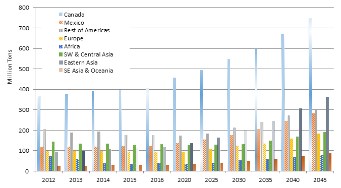
Figure 9. Graph. U.S. Imports by Region of Origin, 2012 — 2045
Nevertheless, Eastern Asia and Southeastern Asia & Oceania remain the fastest growing origins for U.S. imports (4.1 percent CAGR and 4.0 percent CAGR, respectively, over the FAF4 Forecast period). The forecasts suggest the continuing of a long-term trend in rapid manufacturing growth in China, South Korea, Japan, and elsewhere in Eastern Asia for export. Eastern Asia, already a major origin for U.S. imports, will become the second most important origin for U.S. imports by 2045. Southeastern Asia & Oceania starts from a smaller base but grows nearly as fast as Eastern Asia, as manufacturing growth spreads to lower-cost emerging economies such as Vietnam.
| Region Code | Region of Origin | Import Tons, 2012, millions | Import Tons, 2045, millions | Compound Annual Growth Rate, 2012-2045 |
|---|---|---|---|---|
| 801 | Canada | 368 | 746 | 2.2 percent |
| 802 | Mexico | 119 | 283 | 2.6 percent |
| 803 | Rest of Americas | 205 | 304 | 1.2 percent |
| 804 | Europe | 101 | 184 | 1.8 percent |
| 805 | Africa | 77 | 79 | 0.1 percent |
| 806 | SW & Central Asia | 44 | 191 | 0.9 percent |
| 807 | Eastern Asia | 97 | 363 | 4.1 percent |
| 808 | SE Asia & Oceania | 25 | 91 | 4.0 percent |
| Total | 1,136 | 2,241 | 2.1 percent |
The real value of U.S. imports will significantly outpace tonnage growth. Total import value is forecasted to grow from $2.2 trillion in 2012 to $8.1 trillion by 2045, a CAGR of 4.0 percent. This is driven by imports of high-value goods, including electronics and other technology from Eastern Asia and Southeastern Asia & Oceania. The following figure summarizes the trends in import freight flow value growth.
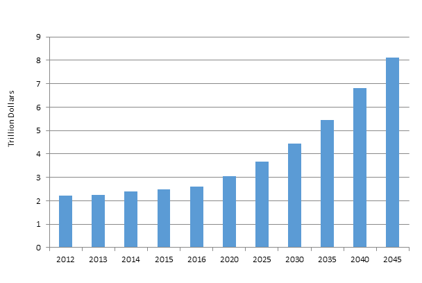
Figure 10. Graph. Real Value of Import Freight Flows, 2012 — 2045
3.2 Optimistic and Pessimistic Alternative Scenarios
The Optimistic and Pessimistic scenario FAF4 forecast data are based on the alternative macroeconomic scenarios described in the Key Assumptions section of this report. The key alternative macroeconomic variables are described in Table 3. These macroeconomic assumptions for the alternative cases are then filtered through regional employment and economic output models, which in turn drive the alternative forecasts of inter-regional freight flows. The process is described in greater detail in the Forecast Methodology section of this document.
The same methodology used to create the Baseline Scenario FAF4 Forecast was followed to create the Optimistic and Pessimistic scenarios forecasts. For the FAF4 Optimistic and Pessimistic forecasts, the appropriate input files were changed to reflect the different levels of employment and output growth captured in the alternative macroeconomic cases.
As previously noted, inputs and processes were adjusted for some commodity classes and origin-destination pairs to more closely calibrate Baseline Scenario flow forecasts with Federal Government data and other third-party macroeconomic and industry growth models. In these cases, the Optimistic and Pessimistic scenarios are adjusted proportionally.
3.2.1 Domestic Optimistic and Pessimistic Scenario Tonnage
The following figures summarize the Optimistic and Pessimistic scenarios compared to the Baseline Scenario. Years 2012-2014 are deemed to be "historical forecast" years; consequently, the deviation from the Baseline Scenario begins in 2015.
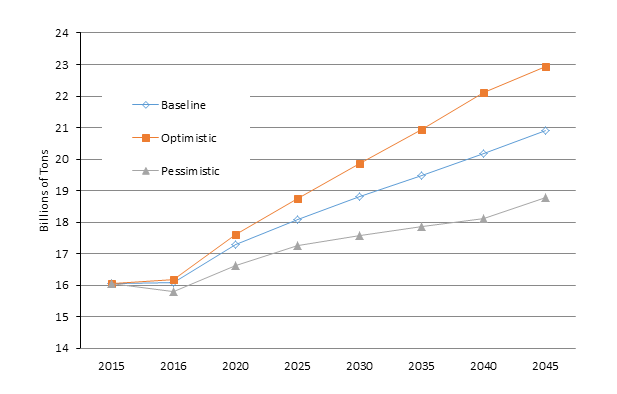
Figure 11. Graph Domestic Tonnages — Baseline, Optimistic, and Pessimistic Scenarios, 2015 — 2045
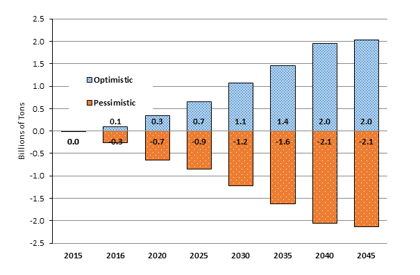
Figure 12. Graph. Domestic Optimistic and Pessimistic Scenario Variations from the Baseline Scenario, 2015 — 2045
In the Optimistic Scenario, total domestic tonnage is expected to grow by 1.3 percent on average per year from 2012 to 2045 as opposed to a 1.0 percent CAGR in the Baseline Scenario. This yields 22.9 billion tons of domestic commodity flow in 2045, 2.0 billion tons higher than in the Baseline Scenario. In the Pessimistic Scenario, total domestic tonnage is projected to grow by 0.7 percent on average per year from 2012 to 2045, resulting in 18.8 billion tons of domestic commodity flow in 2045, 2.1 billion tons less than the Baseline Scenario forecast.
3.2.2 Exports and Imports Optimistic and Pessimistic Scenario Tonnage
In the Optimistic Scenario, total export tonnage is expected to grow by 3.0 percent on average per year from 2012 to 2045 as opposed to a 2.9 percent CAGR in the Baseline Scenario. As a result, export tonnage is estimated to reach 2.3 billion tons in 2045, about 118 million tons higher than in the Baseline Scenario forecast. In the Pessimistic Scenario, total export tonnage is projected to grow by 2.6 percent on average per year from 2012 to 2045, resulting in 2.0 billion tons of exports in 2045, about 169 million tons less than in the Baseline Scenario forecast.
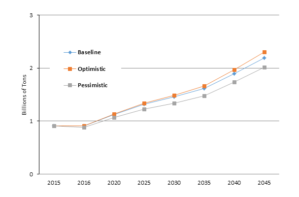
Figure 13. Graph. Export Tonnages — Baseline, Optimistic, and Pessimistic Scenarios, 2015 — 2045
In the Optimistic Scenario, total import tonnage is expected to grow by 3.2 percent on average per year from 2012 to 2045 as opposed to a 2.1 percent CAGR in the Baseline Scenario. Consequently, import tonnage is forecasted to reach 3.2 billion tons in 2045, approximately 932 million tons higher than in the Baseline Scenario forecast. In the Pessimistic Scenario, total import tonnage is projected to grow by 1.1 percent on average per year from 2012 to 2045, resulting in 1.7 billion tons of imports in 2045, about 586 million tons less than in the Baseline Scenario forecast.
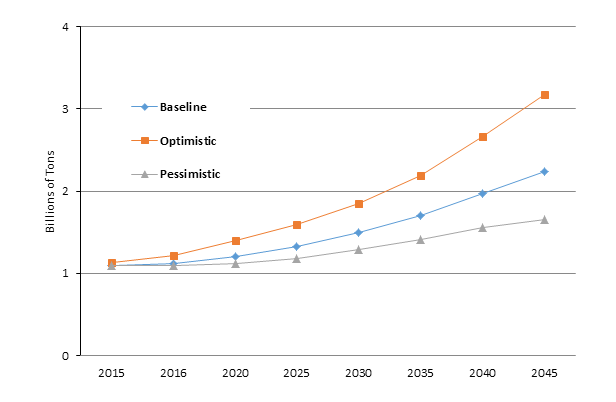
Figure 14. Graph. Import Tonnages — Baseline, Optimistic, and Pessimistic Scenarios, 2015 — 2045
The previous charts illustrate that the Optimistic and Pessimistic scenarios are asymmetrical around the Baseline Scenario forecast. This is due to the fact that the assumptions driving the Optimistic Scenario promote overall consumption and a stronger dollar, thus the higher demand for imports and domestically-produced goods, which limits the amount that can be exported. In the Pessimistic Scenario, reduced demand from lower manufacturing and a weaker dollar eases the need for imports, while significantly reducing the attractiveness and availability of goods for export. Therefore, the impacts of a changing macroeconomic scenario on imports and exports are not necessarily equal.
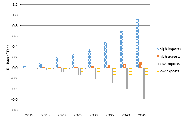
Figure 15. Graph. Variations in Import and Export Tonnage from Baseline, Optimistic, and Pessimistic Scenarios, 2015 — 2045
The three tables that follow summarize the tonnage forecasts across all scenarios by SCTG commodity class from 2012 to 2045. The tables summarize domestic, exported, and imported flows, respectively. In no instance does the Optimistic Scenario or the Pessimistic Scenario result in the changing of the long-term directionality of the growth rate. The dynamics described in the Baseline Scenario summary sub-section are consistent across scenarios. For example, low-tonnage, high-value commodities such as Pharmaceuticals, Precision Instruments, and Transportation Equipment retain their relative rankings in terms of fastest growth over the study time horizon regardless of scenario. The only difference is that the application of optimistic or pessimistic macroeconomic assumptions affects the relative magnitude of growth rates across all SCTG commodity classes.
| Class | Description | 2012 tons (millions) | 2045 tons (millions) | Compound Annual Growth Rate 2012-2045 (percent) |
||||
|---|---|---|---|---|---|---|---|---|
| Source: IHS | ||||||||
| 01 | Live animals/fish | 98.7 | 141.9 | 155.4 | 127.4 | 1.1 | 1.4 | 0.8 |
| 02 | Cereal grains | 870.9 | 1212.1 | 1329.6 | 1086.7 | 1.0 | 1.3 | 0.7 |
| 03 | Other agriculture products | 438.9 | 552.2 | 606.2 | 495.2 | 0.7 | 1.0 | 0.4 |
| 04 | Animal feed | 286.5 | 456.2 | 500.3 | 408.6 | 1.4 | 1.7 | 1.1 |
| 05 | Meat/seafood | 84.9 | 138.9 | 152.3 | 124.3 | 1.5 | 1.8 | 1.2 |
| 06 | Milled grain products | 112.1 | 189.7 | 208.0 | 169.6 | 1.6 | 1.9 | 1.3 |
| 07 | Other foodstuffs | 619.9 | 1041.5 | 1142.7 | 929.8 | 1.6 | 1.9 | 1.2 |
| 08 | Alcoholic beverages | 99.4 | 157.3 | 172.8 | 140.5 | 1.4 | 1.7 | 1.1 |
| 09 | Tobacco products | 3.0 | 0.9 | 1.0 | 0.8 | -3.6 | -3.4 | -4.0 |
| 10 | Building stone | 30.8 | 56.9 | 62.3 | 50.8 | 1.9 | 2.2 | 1.5 |
| 11 | Natural sands | 538.0 | 848.8 | 930.6 | 761.3 | 1.4 | 1.7 | 1.1 |
| 12 | Gravel | 1735.6 | 2434.8 | 2670.2 | 2175.1 | 1.0 | 1.3 | 0.7 |
| 13 | Nonmetallic minerals | 148.1 | 272.3 | 298.8 | 243.1 | 1.9 | 2.1 | 1.5 |
| 14 | Metallic ores | 75.8 | 75.9 | 83.3 | 67.8 | 0.0 | 0.3 | -0.3 |
| 15 | Coal | 996.7 | 539.6 | 593.8 | 497.9 | -1.8 | -1.6 | -2.1 |
| 16 | Crude petroleum | 365.1 | 393.6 | 430.5 | 361.0 | 0.2 | 0.5 | 0.0 |
| 17 | Gasoline | 1043.4 | 960.9 | 1050.6 | 861.6 | -0.2 | 0.0 | -0.6 |
| 18 | Fuel oils | 801.6 | 650.3 | 709.3 | 586.5 | -0.6 | -0.4 | -0.9 |
| 19 | Coal & petroleum prods. | 2223.3 | 3893.1 | 4263.9 | 3508.8 | 1.7 | 2.0 | 1.4 |
| 20 | Basic chemicals | 328.7 | 491.4 | 537.8 | 444.9 | 1.2 | 1.5 | 0.9 |
| 21 | Pharmaceuticals | 16.1 | 40.0 | 43.9 | 35.7 | 2.8 | 3.1 | 2.4 |
| 22 | Fertilizers | 183.3 | 280.8 | 308.0 | 251.7 | 1.3 | 1.6 | 1.0 |
| 23 | Chemical products | 102.0 | 181.4 | 198.8 | 162.1 | 1.8 | 2.0 | 1.4 |
| 24 | Plastics/rubber | 173.6 | 324.8 | 354.9 | 292.4 | 1.9 | 2.2 | 1.6 |
| 25 | Logs | 285.8 | 388.6 | 425.7 | 347.5 | 0.9 | 1.2 | 0.6 |
| 26 | Wood products | 348.8 | 463.1 | 508.0 | 414.0 | 0.9 | 1.1 | 0.5 |
| 27 | Newsprint/paper | 106.5 | 96.7 | 127.2 | 86.3 | -0.3 | 0.5 | -0.6 |
| 28 | Paper articles | 74.8 | 104.7 | 114.9 | 93.4 | 1.0 | 1.3 | 0.7 |
| 29 | Printed products | 37.7 | 41.2 | 45.2 | 36.7 | 0.3 | 0.5 | -0.1 |
| 30 | Textiles/leather | 40.3 | 27.5 | 30.2 | 24.5 | -1.2 | -0.9 | -1.5 |
| 31 | Nonmetal mineral products | 919.6 | 1603.9 | 1758.2 | 1432.9 | 1.7 | 2.0 | 1.4 |
| 32 | Base metals | 296.4 | 435.5 | 477.5 | 388.8 | 1.2 | 1.5 | 0.8 |
| 33 | Articles-base metal | 108.4 | 184.3 | 202.1 | 165.2 | 1.6 | 1.9 | 1.3 |
| 34 | Machinery | 82.9 | 173.7 | 190.4 | 155.6 | 2.3 | 2.6 | 1.9 |
| 35 | Electronics | 50.9 | 113.7 | 124.7 | 101.6 | 2.5 | 2.8 | 2.1 |
| 36 | Motorized vehicles | 119.8 | 168.8 | 185.2 | 150.9 | 1.0 | 1.3 | 0.7 |
| 37 | Transport equipment | 7.7 | 18.6 | 20.4 | 16.8 | 2.7 | 3.0 | 2.4 |
| 38 | Precision instruments | 7.5 | 18.1 | 19.9 | 16.2 | 2.7 | 3.0 | 2.3 |
| 39 | Furniture | 57.3 | 97.4 | 106.9 | 87.0 | 1.6 | 1.9 | 1.3 |
| 40 | Miscellaneous manufacturing | 86.5 | 164.7 | 180.5 | 146.8 | 2.0 | 2.3 | 1.6 |
| 41 | Waste/scrap | 563.0 | 883.6 | 969.6 | 788.3 | 1.4 | 1.7 | 1.0 |
| 43 | Mixed freight | 380.9 | 592.6 | 650.3 | 529.9 | 1.3 | 1.6 | 1.0 |
| 99 | Unknown | 1.3 | 2.0 | 2.2 | 1.8 | 1.3 | 1.6 | 1.0 |
| Class | Description | 2012 tons (millions) | 2045 tons (millions) | Compound Annual Growth Rate 2012-2045 (percent) |
||||
|---|---|---|---|---|---|---|---|---|
| Source: IHS | ||||||||
| Base | High | Low | Base | High | Low | |||
| 01 | Live animals/fish | 0.3 | 0.3 | 0.3 | 0.3 | 0.0 | 0.0 | -0.1 |
| 02 | Cereal grains | 67.1 | 188.1 | 190.9 | 183.8 | 3.2 | 3.2 | 3.1 |
| 03 | Other agriculture products | 61.9 | 204.6 | 210.5 | 198.0 | 3.7 | 3.8 | 3.6 |
| 04 | Animal feed | 26.5 | 56.4 | 57.2 | 55.1 | 2.3 | 2.4 | 2.2 |
| 05 | Meat/seafood | 9.4 | 29.0 | 29.4 | 28.3 | 3.5 | 3.5 | 3.4 |
| 06 | Milled grain products | 3.6 | 9.7 | 9.9 | 9.5 | 3.1 | 3.1 | 3.0 |
| 07 | Other foodstuffs | 21.3 | 78.7 | 79.9 | 76.9 | 4.0 | 4.1 | 4.0 |
| 08 | Alcoholic beverages | 2.1 | 10.3 | 10.4 | 10.1 | 4.9 | 4.9 | 4.8 |
| 09 | Tobacco products | 0.1 | 0.1 | 0.1 | 0.0 | -1.3 | 0.2 | -3.0 |
| 10 | Building stone | 0.3 | 0.6 | 0.6 | 0.6 | 2.0 | 2.1 | 1.8 |
| 11 | Natural sands | 8.9 | 11.7 | 11.7 | 10.9 | 0.8 | 0.8 | 0.6 |
| 12 | Gravel | 2.5 | 3.4 | 3.4 | 3.2 | 0.9 | 0.9 | 0.7 |
| 13 | Nonmetallic minerals | 12.9 | 24.9 | 25.0 | 23.2 | 2.0 | 2.0 | 1.8 |
| 14 | Metallic ores | 26.1 | 60.2 | 60.4 | 55.9 | 2.6 | 2.6 | 2.3 |
| 15 | Coal | 165.5 | 160.8 | 161.3 | 149.3 | -0.1 | -0.1 | -0.3 |
| 16 | Crude petroleum | 3.7 | 23.5 | 23.5 | 21.8 | 5.7 | 5.8 | 5.5 |
| 17 | Gasoline | 33.7 | 63.8 | 64.1 | 59.3 | 2.0 | 2.0 | 1.7 |
| 18 | Fuel oils | 116.8 | 248.5 | 249.5 | 230.9 | 2.3 | 2.3 | 2.1 |
| 19 | Coal & petroleum prods. | 30.2 | 149.2 | 149.7 | 138.6 | 5.0 | 5.0 | 4.7 |
| 20 | Basic chemicals | 42.7 | 128.6 | 129.1 | 119.5 | 3.4 | 3.4 | 3.2 |
| 21 | Pharmaceuticals | 0.8 | 4.1 | 6.8 | 2.3 | 5.2 | 6.8 | 3.3 |
| 22 | Fertilizers | 13.6 | 22.9 | 23.0 | 21.3 | 1.6 | 1.6 | 1.4 |
| 23 | Chemical products | 10.2 | 47.5 | 55.2 | 39.7 | 4.8 | 5.2 | 4.2 |
| 24 | Plastics/rubber | 25.1 | 92.1 | 92.9 | 85.0 | 4.0 | 4.0 | 3.8 |
| 25 | Logs | 10.1 | 33.8 | 33.9 | 31.4 | 3.7 | 3.7 | 3.5 |
| 26 | Wood products | 10.3 | 32.0 | 36.8 | 26.9 | 3.5 | 3.9 | 2.9 |
| 27 | Newsprint/paper | 22.5 | 55.6 | 55.8 | 51.7 | 2.8 | 2.8 | 2.6 |
| 28 | Paper articles | 2.0 | 6.7 | 9.4 | 4.7 | 3.7 | 4.8 | 2.6 |
| 29 | Printed products | 1.3 | 3.6 | 5.9 | 2.0 | 3.2 | 4.7 | 1.4 |
| 30 | Textiles/leather | 5.9 | 18.0 | 29.4 | 9.9 | 3.5 | 5.0 | 1.6 |
| 31 | Nonmetal mineral products | 9.3 | 36.5 | 38.0 | 33.0 | 4.2 | 4.4 | 3.9 |
| 32 | Base metals | 15.3 | 32.2 | 32.3 | 29.9 | 2.3 | 2.3 | 2.1 |
| 33 | Articles-base metal | 9.3 | 29.7 | 41.2 | 27.3 | 3.6 | 4.6 | 3.3 |
| 34 | Machinery | 13.8 | 51.1 | 69.5 | 46.8 | 4.1 | 5.0 | 3.8 |
| 35 | Electronics | 4.2 | 20.1 | 29.7 | 15.9 | 4.9 | 6.1 | 4.1 |
| 36 | Motorized vehicles | 14.8 | 31.0 | 35.1 | 24.6 | 2.3 | 2.7 | 1.6 |
| 37 | Transport equipment | 2.8 | 11.1 | 13.1 | 9.1 | 4.2 | 4.8 | 3.6 |
| 38 | Precision instruments | 0.9 | 7.7 | 12.1 | 4.9 | 6.6 | 8.1 | 5.2 |
| 39 | Furniture | 2.3 | 11.8 | 18.9 | 6.9 | 5.1 | 6.6 | 3.4 |
| 40 | Miscellaneous manufacturing | 1.8 | 11.1 | 15.9 | 9.7 | 5.7 | 6.8 | 5.3 |
| 41 | Waste/scrap | 51.1 | 172.5 | 175.5 | 158.8 | 3.8 | 3.8 | 3.5 |
| 43 | Mixed freight | 1.4 | 5.9 | 9.6 | 3.2 | 4.4 | 6.0 | 2.6 |
| Class | Description | 2012 tons (millions) | 2045 tons (millions) | Compound Annual Growth Rate 2012-2045 (percent) |
||||
|---|---|---|---|---|---|---|---|---|
| Source: IHS | ||||||||
| Base | High | Low | Base | High | Low | |||
| 01 | Live animals/fish | 1.1 | 2.7 | 2.8 | 2.4 | 2.7 | 2.9 | 2.4 |
| 02 | Cereal grains | 8.0 | 18.1 | 19.5 | 16.6 | 2.5 | 2.7 | 2.2 |
| 03 | Other agriculture products | 23.9 | 124.4 | 136.1 | 112.7 | 5.1 | 5.4 | 4.8 |
| 04 | Animal feed | 5.9 | 14.4 | 17.7 | 13.0 | 2.7 | 3.4 | 2.4 |
| 05 | Meat/seafood | 4.6 | 12.5 | 14.5 | 11.1 | 3.1 | 3.5 | 2.7 |
| 06 | Milled grain products | 4.1 | 14.1 | 15.1 | 12.9 | 3.8 | 4.0 | 3.5 |
| 07 | Other foodstuffs | 24.4 | 91.8 | 98.6 | 84.2 | 4.1 | 4.3 | 3.8 |
| 08 | Alcoholic beverages | 9.5 | 56.8 | 61.0 | 52.1 | 5.6 | 5.8 | 5.3 |
| 09 | Tobacco products | 0.1 | 0.1 | 0.1 | 0.0 | 0.0 | 0.8 | -2.2 |
| 10 | Building stone | 0.2 | 1.1 | 1.4 | 1.0 | 5.5 | 6.3 | 5.1 |
| 11 | Natural sands | 2.6 | 3.2 | 4.1 | 2.8 | 0.6 | 1.4 | 0.3 |
| 12 | Gravel | 15.8 | 25.3 | 32.6 | 22.6 | 1.4 | 2.2 | 1.1 |
| 13 | Nonmetallic minerals | 30.5 | 58.7 | 75.4 | 52.4 | 2.0 | 2.8 | 1.7 |
| 14 | Metallic ores | 21.5 | 30.1 | 38.7 | 26.9 | 1.0 | 1.8 | 0.7 |
| 15 | Coal | 7.7 | 34.4 | 44.2 | 30.7 | 4.6 | 5.4 | 4.3 |
| 16 | Crude petroleum | 480.7 | 465.8 | 904.0 | 281.7 | -0.1 | 1.9 | -1.6 |
| 17 | Gasoline | 43.4 | 18.6 | 36.1 | 11.2 | -2.5 | -0.6 | -4.0 |
| 18 | Fuel oils | 67.5 | 53.8 | 104.4 | 32.5 | -0.7 | 1.3 | -2.2 |
| 19 | Coal & petroleum prods. | 59.6 | 135.4 | 174.1 | 120.9 | 2.5 | 3.3 | 2.2 |
| 20 | Basic chemicals | 30.9 | 112.9 | 145.2 | 100.8 | 4.0 | 4.8 | 3.6 |
| 21 | Pharmaceuticals | 2.3 | 12.9 | 16.8 | 6.3 | 5.3 | 6.2 | 3.1 |
| 22 | Fertilizers | 29.4 | 42.2 | 67.8 | 31.7 | 1.1 | 2.6 | 0.2 |
| 23 | Chemical products | 5.9 | 34.1 | 44.0 | 25.4 | 5.4 | 6.3 | 4.5 |
| 24 | Plastics/rubber | 21.6 | 88.1 | 119.9 | 46.2 | 4.3 | 5.3 | 2.3 |
| 25 | Logs | 1.2 | 4.0 | 5.2 | 3.6 | 3.8 | 4.6 | 3.5 |
| 26 | Wood products | 18.0 | 63.2 | 81.7 | 38.9 | 3.9 | 4.7 | 2.4 |
| 27 | Newsprint/paper | 15.5 | 33.5 | 43.1 | 29.9 | 2.4 | 3.1 | 2.0 |
| 28 | Paper articles | 2.0 | 5.6 | 7.3 | 3.2 | 3.2 | 4.0 | 1.4 |
| 29 | Printed products | 1.2 | 2.8 | 3.6 | 1.4 | 2.5 | 3.3 | 0.3 |
| 30 | Textiles/leather | 14.3 | 52.5 | 68.1 | 25.7 | 4.0 | 4.9 | 1.8 |
| 31 | Nonmetal mineral products | 22.5 | 100.1 | 128.7 | 88.4 | 4.6 | 5.4 | 4.2 |
| 32 | Base metals | 36.3 | 82.6 | 102.1 | 74.2 | 2.5 | 3.2 | 2.2 |
| 33 | Articles-base metal | 21.8 | 55.5 | 57.4 | 45.5 | 2.9 | 3.0 | 2.3 |
| 34 | Machinery | 24.4 | 100.8 | 112.3 | 79.3 | 4.4 | 4.7 | 3.6 |
| 35 | Electronics | 15.0 | 68.4 | 82.8 | 45.1 | 4.7 | 5.3 | 3.4 |
| 36 | Motorized vehicles | 28.9 | 68.8 | 111.8 | 32.6 | 2.7 | 4.2 | 0.4 |
| 37 | Transport equipment | 1.0 | 5.6 | 7.6 | 3.5 | 5.2 | 6.2 | 3.8 |
| 38 | Precision instruments | 1.6 | 10.1 | 11.5 | 7.0 | 5.8 | 6.2 | 4.6 |
| 39 | Furniture | 11.4 | 78.4 | 101.7 | 38.4 | 6.0 | 6.9 | 3.8 |
| 40 | Miscellaneous manufacturing | 5.9 | 25.5 | 33.0 | 17.0 | 4.6 | 5.4 | 3.3 |
| 41 | Waste/scrap | 10.7 | 19.8 | 25.4 | 17.6 | 1.9 | 2.7 | 1.5 |
| 43 | Mixed freight | 2.6 | 12.4 | 16.1 | 6.1 | 4.8 | 5.6 | 2.6 |
4 Forecast Methodology
The foundation of the approach to the Freight Analysis Framework (FAF) Fourth Generation (FAF4) Forecasts is the consistency across the forward-looking outlook of macroeconomic, regional, inter-industry, and intra-state forecast models. The economic forecasting models used in this study are built and maintained with a common framework and perspective that provides a comprehensiveness, consistency, and level of detail that are unique for freight transportation forecasting. Most importantly, this means that the detailed freight flow forecasts are derived in a manner consistent with the path of the economy at the national, regional, and sub-state levels.
This section provides a general overview of the forecasting methodology. The following sub-sections will provide a more detailed examination of the steps taken in producing the domestic and international forecasts. Throughout the methodology discussion, third-party tools and databases are referenced. The primary tools and databases used in the FAF4 forecasting process are also described in detail in the Underlying Forecast Drivers: Data Sources section of this document.
The initial calibration in the forecasting process involves two distinct steps. The first is to construct the desired level of geography in the IHS Business Market Insights (BMI) and the Business Transactions Matrix (BTM) forecast databases relative to the 2012 FAF4 base-year database. The creation of the FAF4 regions in these two models is a process of aggregation, grouping the county-level data into the FAF4 regional market definitions, and summing the values.
The second step during this initial stage entails the development of the crosswalk between the North American Industry Classification System (NAICS) industry sector classifications and the two-digit-level Standard Classification of Transported Goods (SCTG) commodity classifications. This is done through a review of existing commodity classification concordance files, which detail the relationships between different combinations of NAICS, SCTG, and Standard Transportation Commodity Classification (STCC) codes at various levels of detail. The crosswalk between industry and commodity classifications is important because it provides the bridge from the value and weight of the physical commodities and products shipped through the transportation system to the industry activity measured by economists on an industry establishment level (typically using the value of output or purchases and/or the associated employment).
The mapping of six-digit NAICS codes to corresponding SCTG codes began with the FAF Third Generation (FAF3) Forecasts concordance table. The FAF3 mapping was then updated so that the concordance table reflects new additions and changes to the code definitions. The Commodity Flow Survey (CFS) microdata file, which also contains NAICS-SCTG relationships, was also employed as a reference where an accurate six-digit NAICS-SCTG mapping could not be determined.
In addition, for international movements, a crosswalk was developed linking SCTG to codes used in the IHS World Trade Service (WTS) model. WTS codes are related to the International Standard Industrial Classification of All Economic Activities (ISIC) system. This crosswalk provides the bridging between the WTS international trade forecasts and the international and cross-border movements in the FAF4 database. A detailed mapping was also completed to match ISIC to the WTS codes, the latter of which have already been updated for concordance with STGC two-digit-level codes (the WTS to SCTG crosswalk appears in the Appendix).
The development of the baseline commodity tonnage forecasts is multi stage. For domestic forecasts, these steps include:
- Establish national control totals by commodity using the Industrial Production Index of the IHS Model of the U.S. Economy (U.S. Macro Model);
- For each commodity, apply specific shipment growth to each CFS region destination from each origin region using the BMI;
- Apply specific purchasing and consumption growth by CFS region and commodity using the BTM;
- Summarize and compare the results from steps 2 and 3 with the national controls in Step 1; and
- Adjust the resulting freight flows so that the volumes correspond with the national control levels:
- For each CFS region and commodity, ratably adjust shipments to match purchases.
- For each commodity, adjust so that national control totals are satisfied.
For international forecasts, these steps include:
- Using the BTM and the BMI data, respectively, grow imports and exports by FAF region for all commodities by Federal Highway Administration (FHWA)-defined United States (U.S.) Gateway and World Region, and applying WTS forecasts;
- Establish national import and export control numbers for each commodity by FHWA-defined U.S. Gateway and World Region using the WTS;
- Ratably adjust the import and export forecasts in Step 1 with national controls for each in Step 2; and
- Adjust 2013 and 2014 international forecasts to be consistent with provisional Federal Government trade data.
The following sub-sections provide greater detail on the domestic and international freight forecasting methodologies, reconciling short-term forecasts (2013 and 2014) with actual provisional data, the conversion of value forecasts to real dollars, the development of alternative scenarios, and descriptions of various case-by-case adjustments to calculating forecasts in certain cases.
4.1 Domestic Freight Forecast Methodology
The first step in creating the forecast of the FAF4 database is to extract the county-level employment and the U.S. dollar value of output information, by 6-digit NAICS code, from the BMI database. The BMI database covers each of the forecast years from 2012 to 2040. BMI is extended to 2045 for the purposes of this project. The BMI database is described in detail in the Underlying Forecast Drivers: Data Sources section of this report.
The employment data from the BMI is then matched to the SCTG categories, and aggregated to the 2-digit SCTG level to conform to the FAF4 2012 base-year database. The concordance table identifying the relationships between NAICS and SCTG coding systems is used in this processing. Extensive cross-referencing is required to ensure that all detailed NAICS industry categories in the BMI are assigned to a SCTG commodity class code, and also that all SCTG commodity class codes in the FAF4 data are assigned to a NAICS industry sector classification.
Concurrent with the extension of the BMI output and employment forecasts to 2045, county-level data is aggregated to match the geographic market region definitions used in the 2012 FAF4 base-year database. The counties are mapped to the FAF4 geographic regions using the definitional assignments provided by the FHWA. The output and employment data are then converted to growth rates. The results are cross-checked and verified against the growth rates for the individual constituent counties.
The independent forecast variables include data from the BTM database, which are described in detail in the Underlying Forecast Drivers: Data Sources section of this report. The BTM Input/Output (I/O) tables require a similar methodology for translation of the NAICS industry classification codes to SCTG commodity category codes, and the county-level geography to the FAF4 geographic market regions. Again, minor adjustments to the NAICS-to-SCTG relationships are necessary to insure that all SCTG categories are assigned to NAICS industry categories, for example:
- NAICS 212322 → 25 percent to SCTG 11 & 75 percent to SCTG 12
- NAICS 211111 → 45 percent to SCTG 16 & 55 percent to SCTG 19
- NAICS 324110 → 26 percent to SCTG 17, 25 percent to SCTG 18 & 50 percent to SCTG 19
The total domestic shipment volumes are then projected out through the forecast horizon using the forecast information from the BMI, converted to annual growth rates. The result is a table that shows, for each of the forecast years, the shipment tonnage for each CFS region-to-region SCTG commodity flow.
The BTM I/O data is then integrated with the 2012 base-year FAF4 database, so that for each origin region-SCTG commodity combination there is a complete set of purchased (consumed) goods associated with SCTG commodity volumes. The base-year purchase volumes are then forecasted for each year of the forecast period using the forecasted growth rates in the BTM.
At this point, a national-level freight forecast, based on the most recent U.S. economic data from the U.S. Macro Model, is employed to establish aggregate-level benchmark freight volumes for each SCTG commodity class. The total 2012 base-year FAF4 freight flows, by SCTG commodity, are then initially forecasted using the national-level forecasts of output and consumption.
Once these national-level benchmark values are established, the last step is to reconcile and rebalance the original BMI-based region-to-region shipment forecast and the BTM-based region-to-region purchases forecast. This iterative process yields the detailed CFS-market-to-CFS market commodity flow volumes, which are adjusted to and constrained by the national benchmarks established using the U.S. Macro Model.
Lastly, annual growth rates are reviewed against various Federal Government and third-party industrial production and transportation flow benchmarks to validate the forecasts. As will be described later in this section, several adjustments were applied to flows at various dimensions (e.g. the SCTG level, origin-destination level, etc.) where the overall forecasting process produced results substantially different from the appropriate Federal Government and/or third-party benchmarks.
4.2 International Freight Forecast Methodology
The procedure for forecasting the international components of the FAF4 data is similar in nature to that which is used for the domestic traffic, but some adjustments are required due to the different underlying growth drivers for international business transactions and the additional gateway or port market definitional dimension that must be incorporated. The process of producing the international forecasts treats the import and export portions of the international data separately, as the treatment of suppliers and consumers is asymmetrical with respect to the level of detail available on each end of the transaction (i.e., much more detail is available on the U.S. end of the shipment).
In addition, for the forecast years of 2013 and 2014, actual provisional import and export data is currently available. It is important for the forecasts to correctly reflect existing data as best as possible. To that end, the international freight forecasts use additional inputs from the U.S. Census and from other relevant Federal Government sources to produce international flows consistent with trade data for those two years. The latest "forecast" year of 2014 is used as the driver of the international forecast so that movements appearing in the 2014 data will continue in the forecast whether or not they appear in the FAF4 2012 base-year database. The specific process used to make assignments in 2013 and 2014 international data is detailed later in this report.
The base-year FAF4 data set is maintained throughout the processing in separate files for domestic, import, and export freight flows. Unlike the domestic data, the international records also contain the gateway or port market identifying where flows enter or exit the US. The originating foreign geographic market for imports and the foreign destination geographic market for exports is identified by the foreign region in the base-year 2012 FAF4 database and in the forecasts (as well as for the adjusted forecasts for new flows appearing in provisional actual data for 2013 and 2014).
Individual commodity growth rates of U.S. imports and U.S. exports, taken from the WTS model, are then applied to the FAF4 base-year international data set to obtain forecast flows by the gateway/foreign geographic regional market/SCTG commodity class combination. The processes and methodologies underlying WTS are described in the Underlying Forecast Drivers: Data Sources section of this report.
To apply the WTS to the FAF4 2012 base-year database, the commodity classifications of the WTS have been translated to SCTG commodity classes. The relationships between the WTS and the SCTG commodity codes are listed in the Appendix of this document. In addition, the geographic country and regional market areas used in the WTS are translated to match those used in FAF4.
With the necessary commodity class and geographic regional market mappings complete, export volume growth is then forecasted by regional market and commodity using BMI export data and WTS foreign import purchases data. For U.S. international import volume growth, also by geographic regional market and SCTG commodity class, the shipment-level import freight flow forecast are calculated as a function of the WTS import forecast and the demand for purchases forecasted in the BTM.
Consistent with the domestic forecasts, national-level constraints by SCTG commodity class are applied in an iterative process. Import shipment-level forecasts are controlled by purchases, and export purchases are controlled by shipments. Once the national-level constraint derived using the WTS is applied, a similar process is completed for each port/SCTG commodity class pair. The resulting file yields total tonnage for each forecast year for each regional market-gateway/region-SCTG commodity class combination.
After employing quality controls, including any adjustments determined through the validation process, the output includes international forecasts formatted with annual growth changes for each SCTG commodity class, gateway and SCTG commmodity class, and foreign geographic region market and SCTG commodity class.
4.3 Development of 2013 and 2014 International Flows
In order to produce forecasts consistent with known values, additional processing is employed to 2013 and 2014 forecast years for international movements. FAF4 forecast years 2013 and 2014 should be consistent with dollar value and tonnage data derived from Customs and trade data information, where available, that are published by various Federal Government agencies5 along the following measures:
- External geography
- U.S. port aggregated to the corresponding FAF district
- Commodity
- Ultimate U.S. internal origin or destination
Movements that occur in the base-year 2012 FAF4 database are adjusted to match the known 2013 and 2014 totals in the FAF4 forecast years. Those 2014 totals are then used as the base for the outer-year forecasts.
Movements that do not occur in the base-year 2012 FAF4 database but are known to have occurred in 2013 or 2014 due to their presence in other Federal Government agency data publications are added so that the totals by port, commodity, and geography are consistent with known values. The trade data is available separately as commodity totals by U.S. port and Customs district, totals by commodity and external trading partner, and totals by commodity and inland origin and destination. A process was created to reconstruct these new flows identified in more recent provisional records by country-commodity-port-inland origin/destination such that the resulting 2013 and 2014 data are consistent with totals across all dimensions and forecasted into the future.
For overland flows, the Bureau of Transportation Statistics (BTS) provides information on cross-border shipments by truck, rail, and pipeline, in terms of declared value (in U.S. dollars) at customs inspection points on the border. Information on export shipments includes U.S. state of origin, crossing point, and external destination and (separately) U.S. origin, commodity, and destination. For imported shipments, U.S. state of destination and the crossing point are shown. In addition, physical volume (tons) and values are reported for these shipments.
For those movements where dollar value is available but without corresponding weight information, tonnage is computed using historical ratios of weight to value. This process includes creating a translation table relating the Harmonized Code (in which the aforementioned data are recorded) to corresponding classifications in U.S. Customs data, from which dollar-ton conversions can be derived. Data published by the U.S. Army Corps of Engineers and the U.S. Office of Airline Information is also leveraged for developing waterborne and air cargo tonnage estimates, respectively. Where possible, this conversion relies on the unit counts of imports and exports. For commodities where unit weight varies widely, this conversion relies on a table of product values; however, adjustments are made in some instances where a dollar value is deemed more appropriate for import/export trade in a given commodity. Unit counts are added for truck and rail using averages from data exchange or commodity specific defaults.
4.4 Real Value (Constant Dollar) Forecast Methodology
The goal of this exercise is to provide a real or constant dollar estimate of value for all FAF4 Forecast years. That is, future FAF4 value forecasts should exclude the effects of inflation. For this study, a simple, striaghtforward approach was adopted, where the real or constant dollar value is the forecasted tonnage multiplied by the 2012 dollar price over the entire time horizon. Therefore, the driver of long-term value flows is directly associated tonnage growth, exclusive of inflation or any other future price changes.
4.5 Addressing Structural Changes to Historical Trends
The FAF4 forecasting process is based primarily on 2012 data (with adjustments to international flows from available 2013 and 2014 provisional data); with growth rates applied using various third-party macroeconomic and trade forecasts. There are cases where the historical data is not as strong a basis for likely future flows. Moreover, there are known current and future structural changes affecting domestic and international freight flows but for which impacts are highly uncertain.
The approach employed in this study to acccount for potential structural changes to historical trends is to evaluate them on a case-by-case basis with the aid of various macroeconomic and industry data, tools, and insight. This process is undertaken during the forecasting phase in the validation of model output for consistency with Federal Government data, the U.S. Macro Model, and other IHS industry-specific forecasting products.
Adjustments to the overriding methodology are applied only for those flows for which future structural changes are well known and likely impacts can be reasonably inferred. For example, it is known that the Panama Canal expansion will occur and may impact historical commodity trade volumes and routing. However, the impacts are highly uncertain and likely asymmetrical across commodity classes and trade lanes. In theory, the ability for larger maritime vessels to transit the Panama Canal will lower freight rates per unit of cargo due to scale economies (all else equal), potentially increasing demand for traded goods (due to lower transportation costs) and/or altering mode or route choices. However, the outlook is fluid and substantial uncertainties include, but are not limited to:
- Competitive responses (e.g., by port terminal operators on the Pacific Coast and railroads);
- The long-term development of landside infrastructure at North American ports;
- Advancements in maritime vessel technology incompatible with new Panama Canal dimensions6; and
- The evolution of industry supply chain strategies and ocean carrier operating strategies.
To illustrate this approach; the cases of crude petroleum and liquefied natural gas (LNG) are compared. While some larger oil tankers may pass through the expanded Panama Canal, this alone is unlikely to significantly affect crude oil flows and routes. This is because high-volume waterborne crude oil transportation tends to employ vessels that are too large even for the expanded Panama Canal locks. Therefore, there is no reason to adjust crude petroleum flow forecasts until additional factors suggest otherwise. Meanwhile there is historically limited LNG trade from the U.S. East Coast to Asia. However, the Panama Canal expansion will enable larger gas tankers to move LNG from the U.S. Gulf Coast and possibly the U.S. Atlantic Coast to Asia, potentially making U.S. producers cost competitive in major Eastern Asia markets. Moreover, the Federal Government has approved natural gas liquefaction plant plans and export permits for numerous would-be exporters. The FAF4 forecast methodology does not capture the likely magnitude of growth or the development of new trade lanes for the commodity class corresponding to natural gas (SCTG 19). Therefore, adjustments are made to calibrate import and export trade forecasts with IHS natural gas trade forecasts.
4.6 Special Forecasting Categories
In several instances the normal forecasting methodology yielded results which lack consistency with either the underlying fundamentals of a given commodity class, or broke with long-standing trends for which inadequate evidence exists. In these special circumstances an alternative methodology was used to achieve consistency between the FAF4 Final Forecast and commodity class fundamentals and trends.
The primary inputs to the forecasting methodology are macroeconomic drivers, which are translated by the BMI indices into FAF-region employment and output growth data. Where the BMI-driven forecasts for a given commodity class deviated significantly from Federal Government and/or other third-party industry specific forecasts, alternative IHS industry-specific forecasts are substituted. The following special categories summarize these changes:
- Domestic agricultural commodity class (SCTGs 1, 2, 3, 4, 22) growth rates are realigned to match forecasts from the IHS Agriculture group. Transportation demand is derived from these forecasts, which generally predict a continuation in increasing yield per acre and decreasing planted acreage.
- Imported and domestic Gravel and Crushed Stone (SCTG 12) volumes have been adjusted downward to reflect reduced construction and related industrial activity.
- Natural Sands and Gravel and Crushed Stone (SCTGs 11, 12) growth at specific origins have been revised downward as the BMI drivers, employment and output, did not accurately reflect transportation activity.
- Energy commodities (SCTGs, 15, 16, 17, 18, 19) are realigned to reflect forecasts from the IHS Energy group. The changes primarily reflect a more optimistic outlook for domestic natural gas tonnage and a more pessimistic outlook for domestic coal tonnage. Expected structural changes in trade patterns are reflected in export and import forecasts for several origin-destination pair and commodity class combinations.
- Fertilizers (SCTG 22) domestic tonnage growth originating in Texas and Louisiana has been increased as major production capacity expansion is expected. The extent of this growth was not fully captured in the BMI employment and output forecast growth rates. This increase in production is largely due to low domestic raw energy feedstock prices, primarily low natural gas prices.
- Plastics (SCTG 24) domestic tonnage growth originating in certain FAF zones in Texas, Louisiana, and West Virginia has been increased as major production capacity expansion is expected. The extent of this growth was not fully captured in the BMI employment and output forecast growth rates. This increase in production is largely due to low domestic raw energy feedstock prices, primarily low domestic natural gas liquids prices.
- Domestic forestry related and paper products (SCTGs 25, 26, 27, 28, 29) have been adjusted downward to reflect observed trends in lumber supply and paper demand. The reported output of pulp and paper mills is analyzed to inform the forecasts. Lower production growth in wood and lumber is likely to continue through the forecast horizon, while increased digitization of newsprint and packaging efficiency will continue to slow demand for paper products.
- Domestic Motorized Vehicles (SCTG 36) forecasts are adjusted downward to reflect forecasts from the IHS Automotive group, which show a diminishing growth rate in vehicle demand.
- Domestic Other Manufacturing and Mixed Freight (SCTGs 40, 43) are adjusted downward to more accurately reflect manufacturing and consumption growth patterns.
- General algorithms are developed to mitigate abnormally and inexplicably high (or low) domestic growth rates. These algorithms address two major factors contributing to outlier results: (a) where industry growth diverges from traffic growth (e.g., the headquarters effect) and (b) out-year extrapolation of high early-year growth.
5 Underlying Forecast Drivers: Data Sources
The following sections of this report summarize the various IHS databases and services that are used in constructing the Freight Analysis Framework (FAF) Fourth Generation (FAF4) Forecast database. These include the aforementioned United States (U.S.) Macro Model, Business Market Insights (BMI), Business Transactions Matrix (BTM), World Trade Service (WTS), and other U.S. national and regional economic forecasts.
5.1 IHS Model of the U.S. Economy
The IHS flagship model of the U.S. economy integrates modern economic theory and behavior in an analytical tool that is widely used in forecasting, assessing derivative risks, and evaluating policy alternatives. The theoretical structure of the IHS Model of the U.S. Economy, or the "U.S. Macro Model", strives to incorporate the best insights of many theoretical approaches to the business cycle: Keynesian, Neoclassical, monetarist, supply-side, and rational expectations. It embodies major properties of the Neoclassical growth models developed by Robert Solow; thus ensuring that short-run cyclical developments will converge to robust long-run equilibrium.
In growth models, the expansion rate of technical progress, the labor force, and the capital stock determine the productive potential of an economy. Both technical progress and the capital stock are governed by investment, which in turn must be in balance with post-tax capital costs, available savings, and the capacity requirements of current spending. As a result, monetary and fiscal policies will influence both the short- and the long-term characteristics of such an economy through their impacts on national saving and investment.
A modern model of output, prices, and financial conditions is melded with the growth model to present the detailed, short-run dynamics of the economy. In specific goods markets, the interactions of a set of supply and demand relations jointly determine spending, production, and price levels. Typically, the level of inflation-adjusted demand is driven by prices, income, wealth, expectations, and financial conditions. The capacity to supply goods and services is keyed to a production function combining the basic inputs of labor hours, energy usage, and the capital stocks of business equipment and structures, and government infrastructure. The "total factor productivity" of this composite of tangible inputs is driven by expenditures on research and development that produce technological progress.
Prices adjust in response to gaps between current production and supply potential and to changes in the cost of inputs. Wages adjust to labor supply-demand gaps (indicated by a demographically adjusted unemployment rate), current and expected inflation (with a unit long-run elasticity), productivity, tax rates, and minimum wage legislation. The supply of labor positively responds to the perceived availability of jobs, to the after-tax wage level, and to the growth and age/gender mix of the population. Demand for labor is keyed to the level of output in the economy and the productivity of labor, capital, and energy. Tempering the whole process of wage and price determination is the exchange rate; a rise in this rate signals prospective losses of jobs and markets unless costs and prices are reduced.
For financial markets, the model predicts interest rates, exchange rates, stock prices, loans, and investments interactively with the preceding Gross Domestic Product (GDP) and inflation variables. The Federal Reserve sets the supply of reserves in the banking system and the fractional reserve requirements for deposits. In the Model, "monetary policy" is defined by a set of targets, instruments, and regular behavioral linkages between targets and instruments. The model user can choose to define unchanged monetary policy as unchanged reserves, or as an unchanged reaction function in which interest rates or reserves are varied in response to changes in economic indicators such as the price level and the unemployment rate.
The Model captures the full simultaneity of the U.S. economy, forecasting over 1,400 concepts spanning final demands, aggregate supply, prices, incomes, international trade, industrial detail, interest rates, and financial flows. The structure of the interactive sectors is summarized in the diagram below. The following discussion presents the logic of each sector and significant interactions among sectors.
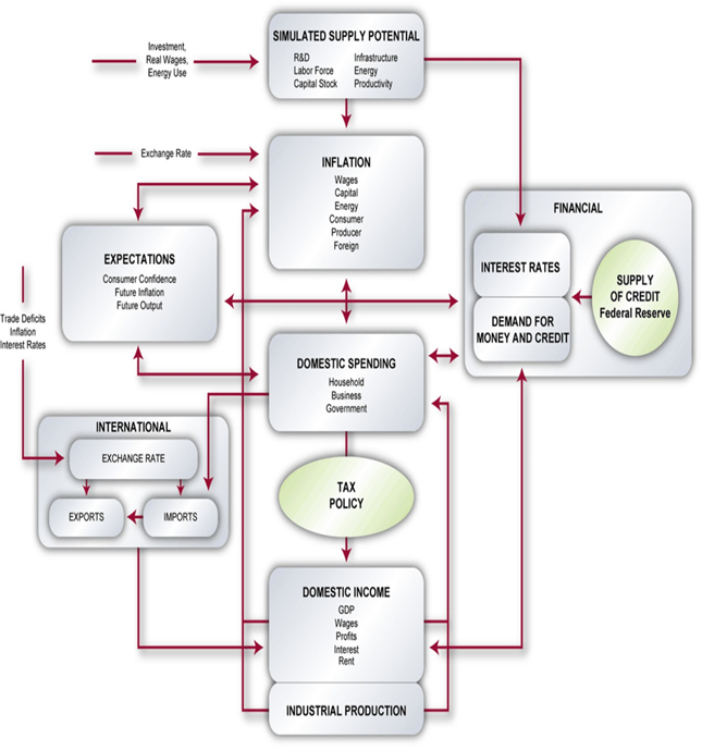
Figure 16. Chart. Overview of the IHS Model of the U.S. Economy
Source: IHS
Consumer Spending: The domestic spending, income, and tax policy sectors model the central circular flow of behavior as measured by the national income and product accounts. Consumer spending is divided into 11 durable goods categories, 9 nondurable goods categories, and 16 service categories. Real consumption expenditures are motivated by real income and the user price of a particular category relative to the prices of other consumer goods. Durable and semi-durable goods are especially sensitive to current financing costs, and consumer speculation on whether it is a "good time to buy." The University of Michigan Survey of Consumer Sentiment monitors this last influence, with the index itself modeled as a function of current and lagged values of inflation, unemployment, and the prime rate.
Business Investment: Business spending includes 19 fixed investment categories. Each equipment and structures spending category is determined by its specific effective post-tax capital costs, capacity utilization, and replacement needs. The cost terms are sophisticated blends of post-tax debt and equity financing costs (offset by expected capital gains) and the purchase price of the investment good (offset by possible tax credits and depreciation-related tax benefits). This Neoclassical structure builds upon the work of Dale Jorgenson, Robert Hall, and Charles Bischoff.
Residential Investment: The residential investment sector of the model includes two categories of housing starts (single and multi-family starts) and three housing sales categories (sales of new and existing single family units, and new single family units for sale), as well as five GDP account categories. The housing sector of the Model explains new construction as a decision primarily based on the after-tax cost of home ownership relative to disposable income. The equations also include a careful specification of demographic forces related to home ownership.
Government: The government sector is largely exogenous (user-determined) at the Federal level and endogenous (equation-determined) at the State and local level. Because of a large and growing deficit, no constraints are imposed on Federal spending. This contrasts sharply with the State and local sectors, where legal requirements for balanced budgets mean that declining surpluses or emerging deficits produce both tax increases and reductions in spending growth.
Incomes: Domestic spending, adjusted for trade flows, defines the economy's value-added or gross national product (GNP) and GDP. Because all value-added must accrue to some sector of the economy, the expenditure measure of GNP also determines the Nation's gross income. The distribution of income among households, business, and government is determined in the Tax Policy and Domestic Income sectors of the model. Every pre-tax income category except for corporate profits is determined by some combination of wages, prices, interest rates, debt levels, and capacity utilization or unemployment rates. Profits are one of the most volatile components of GNP on the income side. When national spending changes rapidly, the contractual arrangements for labor, borrowed funds, and energy imply that the return to equity holders is a residual that will soar in a boom and collapse in a recession. The model reflects this by subtracting each non-profit income item from national income to solve for profits.
Taxes: Since post-tax rather than pre-tax incomes drive expenditures, each income category must be taxed at an appropriate rate; therefore, the model therefore tracks personal, corporate, payroll, and excise taxes separately. Users may set Federal tax rates; tax revenues are then simultaneously forecast as the product of the rate and the associated pre-tax income components. However, the model automatically adjusts the effective average personal tax rate for variations in inflation and income per household, and the effective average corporate rate for credits earned on equipment, utility structures, and research and development.
International: The international sector is a critical, fully simultaneous block that can either add to or divert strength from the central circular flow of domestic income and spending. Depending on the prices of foreign output, the U.S. exchange rate, and competing domestic prices, imports capture varying shares of domestic demand. Depending on similar variables and the level of world gross domestic product, exports can add to U.S. production. The exchange rate itself responds to international differences in inflation, interest rates, trade deficits, and capital flows between the United States and its competitors. Eight aggregate-level categories of goods and two service categories are separately modeled for exports and imports, with one additional category for oil imports.
Investment income flows are also explicitly modeled. The stream of huge current account deficits incurred by the United States has important implications for the U.S. investment income balance. As current account deficits accumulate, the U.S. net international investment position and the U.S. investment income balance deteriorate. U.S. foreign assets and liabilities are therefore included in the model, with the current account deficit determining the path of the net investment position.
Financial: The use of a detailed financial sector and of interest rate and wealth effects in the spending equations recognizes the importance of credit conditions on the business cycle and on the long-run growth prospects for the economy. Interest rates, the key output of this sector, are modeled as a term structure, pivoting off the Federal Funds Rate. The Federal Funds Rate is determined in response to changes in such policy concerns as inflation and unemployment. Longer-term interest rates are driven by shorter-term rates as well as factors affecting the slope of the yield curve. In the IHS Model, such factors include inflation expectations, government borrowing requirements, and corporate financing needs.
Inflation: Inflation is modeled as a carefully controlled, interactive process involving wages, prices, and market conditions. The principal domestic cost influences are labor compensation, nonfarm productivity (output per hour), and foreign input costs; the latter are driven by the exchange rate, the price of oil, and foreign wholesale price inflation. Excise taxes paid by the producer are an additional cost fully fed into the pricing decision. This set of cost influences drives each of the industry-specific producer price indexes, in combination with a demand pressure indicator and appropriately weighted composites of the other producer price indexes. In other words, the inflation rate of each industry price index is the reliably weighted sum of the inflation rates of labor, energy, imported goods, and domestic intermediate goods, plus a variable markup reflecting the intensity of capacity utilization or the presence of bottlenecks.
Supply: The first principle of the market economy is that prices and output are determined simultaneously by the factors underlying both demand and supply. In the Model, aggregate supply, or potential GDP, is estimated by a Cobb-Douglas production function that combines factor input growth and improvements in total factor productivity. Factor input equals a weighted average of labor, business fixed capital, public infrastructure, and energy provided by the energy sector. Total factor productivity depends upon the stock of research and development capital and trend technological change. Taxation and other government policies influence labor supply and all investment decisions, and thus potential supply. The growth of aggregate supply is the fundamental constraint on the long-term growth of demand. Inflation, created by demand that exceeds potential GDP, raises credit costs and weakens consumer sentiment, thus putting the brakes on aggregate demand.
Expectations: Expectations influence several expenditure categories in the Model, but the principal nuance relates to the entire spectrum of interest rates. Shifts in price expectations or the expected capital needs of the government are captured through price expectations and budget deficit terms, with the former affecting the level of rates throughout the maturity spectrum and the latter affecting intermediate- and long-term rates, and thus affecting the shape of the yield curve. On the expenditure side, inflationary expectations affect consumption via consumer sentiment, while growth expectations affect business investment.
5.2 IHS U.S. Regional Economic Forecasting Models
The IHS approach to state and metropolitan area models represents a significant departure from most previous multiregional modeling and forecasting efforts. Most other regional models are constructed as proportions of the US. In the IHS Economics system, however, each area is modeled individually and then linked into a national system. Thus, our models do not forecast regional growth as simple proportions of U.S. totals, but focus on internal growth dynamics and differential business cycle response. This approach is referred to as "top-down bottom-up." It contrasts sharply with pure share (top-down) models, and models which are not linked to a national macroeconomic model (bottom-up), and contains the best of both approaches.
Our basic objective is to project how regional activity varies, given an economic environment as laid out by macroeconomic and industry forecasts. In order to do this; two key phenomena must be explained:
- Why states react differently from one another over the business cycle and
- Why states grow or decline relative to each other over the longer run.
These issues are addressed using information about detailed industrial mix, interindustry and interregional relationships, productivity and relative costs, and migration trends.
5.2.1 Core Economic Forecasting Module
The State and Metropolitan Statistical Area (MSA) models are econometric and have a quarterly periodicity. Consequently, each model is able to capture the full business cycle behavior of the economy, including the timing and amplitude of the turning points.
Another general characteristic of the models is that they are policy sensitive — they respond to changes in tax rates, military spending, utility costs, etc. There are a number of reasons for this sensitivity, and these will be highlighted in the description below. A few of these reasons are the following:
- Each state is modeled individually, with different model structures specified according to the characteristics of the state;
- National policy is explicitly captured; and
- The comparative advantage of one state over another is explicitly modeled using relative cost variables.
The three major components of the approach are summarized below:
- The major linkages among the models occur in the economic base or export sectors. These are primarily agriculture, mining, the Federal Government, and most manufacturing industries. In a few states, banking, insurance, or services (hotels) sectors also can be classified as export sectors. For the most part, these industries serve national rather than local markets or are not dependent upon the local market. On the other hand, the income generated from these sectors provides one of the major stimuli to the local economy. The local growth and decline of these sectors has a lot to do with the economic health of the region.
- The local economy is composed of construction, transportation, utilities and communications, finance, insurance, and real estate, wholesale and retail trade, services, and state and local government. The major driving forces in this part of the economy are local in nature. The income generated by the export sectors circulates and multiplies through the local economy and generates the greater part of regional employment. These interactions and simultaneities can only be captured in an independent model.
- In the demographic sector, net migration is driven by economic conditions. The principal assumption here is that people follow jobs and higher incomes rather than vice-versa. This does not mean that nonpecuniary determinants of migration do not exist. However, these are either fixed (climate and landscape) or vary only slowly (urbanization) or are special in nature (the ability to sell homes and retire to Sunbelt areas). The important thing is to provide the correct direction of causality. Demographic factors are most important on the consumption side of the regional economy. They are a significant factor in housing, retail sales, autos, etc., and the relationships are captured in the models. Population is also an important long-term determinant of the size of such sectors as state and local government.
Manufacturing, for example, is a prime determinant of utilities and transportation employment. In highly industrialized states, it has an effect on almost every nonmanufacturing support sector. In certain western states; on the other hand, it is agriculture or mining which are important export sectors. The appropriate export sector is explicitly represented in the equation and, in this way, the second effects of a new plant, a new mine or increased acreage is directly captured in the nonmanufacturing sectors. Since nonmanufacturing has explicit feedbacks unto itself, the third- and fourth-order effects are also captured. It is a truly dynamic and policy sensitive equation structure.
5.2.1.1 Labor Costs
When real wages are high and/or rising rapidly, then the tendency of business, government, and other organizations is to hold employment down as much as possible. The reverse holds true when real wages are low or falling rapidly. In the manufacturing sector, wage costs were shown to be one of the principle determinants of business location decisions. In the nonmanufacturing support sectors, this is reflected in the level rather than the location of employment. Thus, employment is inversely proportional to real wage costs. Real wages enter many of the nonmanufacturing employment equations. For forecast purposes, this wage rate is related to the appropriate national variable and the growth rate of the sector itself.
5.2.1.2 National Conditions
The national economy is reflected in three areas in the nonmanufacturing sectors. First, certain macroeconomic conditions affect local activity significantly, even nonmanufacturing. The best example of this is credit availability. Tight credit conditions with high interest rates have an adverse impact on local construction activity, sales of autos, and sales of other durables and the like. Thus, when money is tight, employment in construction and in wholesale and retail trade is adversely affected. The opposite holds true during periods of easy money and low interest rates.
The second class of national variables includes those factors which reflect nationwide trends. An example of this is the trend towards an increasingly larger services sector. Capturing this secular trend is sometimes difficult when one uses only local variables in the nonmanufacturing equations. Thus, the usual assortment of local variables — income, populations, wages costs, etc. — is sometimes supplemented by the ratio of sector employment to total employment at the national level. This is not a "shift-share" relationship. It is used to supplement, not supplant, local activity variables. The elasticity on the national series is uniformly lower than the elasticity on the local variables, and it is simply reflecting gradual long-term changes in the nation’s employment structure. The local variables remain the main drivers of the local economy.
5.2.1.3 Demographics — Components of population change
- Births
- Deaths
- Net migration
A few decades ago, natural increase accounted for 68 percent of population growth nationwide, but in a number of fast-growing states in the South and West, net migration accounted for over half of the gain, making interstate mobility an important determinant of state population growth. In addition, within the last 10 years, migration patterns have become even greater influences in these states — both through accelerated interstate population flows, as well as international migration. The IHS econometric analysis of net migration is based upon economic determinants differentiates its forecasts from the U.S. Census Bureau's trended state projections.
5.3 IHS Business Market Insights (BMI)
The BMI database, formerly known as the Business Demographics Model, contains a consistent set of historical statistical estimates and forecasts by industry sector and by geographic region. The statistics include the number of business establishments, employees, and sales by industry. Industry aggregation levels include the sub-sectors and the 4-, 5-, and 6-digit classifications in the North American Industry Classification System (NAICS) codes. The model specifically forecasts variables at the county level. Other geographic levels are created by combining, aggregating, or splitting data from this level. All business demographics modeled databases are designed to meet two key criteria. First, they must reflect economic activity that is consistent with actual information available at this level of geography. Second, they must agree with published values for national and state employment, establishment, and sales data.
The business demographic concepts included in the BMI include:
Number of Employees
- Total
- By Industry
- By Occupation Group
- By Geographic Area
- By Business Size (Non-standard, and not used in the FAF4 Forecasts)
Number of Business Locations
- By Industry
- By Business Size (Non-standard, and not used in the FAF4 Forecasts)
- By Geographic Area
Industry Segments
- 4-Digit NAICS Code
- 5-Digit NAICS Code
- 6-Digit NAICS Code
Business Size Segments (Non-standard, and not used in the FAF4 Forecasts)
- 1 to 4 Employees
- 5 to 9 Employees
- 10 to 19 Employees
- 20 to 49 Employees
- 50 to 99 Employees
- 100 to 249 Employees
- 250 to 499 Employees
- 500 to 999 Employees
- 1000 Employees or More
Geographic Segments
- Geographic Segments
The following discussion describes the data and estimation techniques used in the BMI.
5.3.1 Data
Every BMI forecast starts with at least one observation of activity at the level of geography of interest. This observation, generally collected by a government agency, is treated as an "actual" measurement of the economic activity within a given geographic area. In fact, this observation really is an estimate of activity. The government surveys a percentage of employers within the region and then imputes the value for the region as a whole from this sample. As with any estimate, these "actual" observations may deviate from the "truth." However, as the size of the geographic area increases, so too does the accuracy of the estimate (due to the law of averages). This is why the sum of our county level forecasts will always add up to a measurement or an estimate of state and national level activity.
Several data sources were used as a basis for the first round model of county employment and establishments. U.S. County Business Patterns (CBP) data provides a series of county-level employment and establishments from 1980 to 1996 at the four-digit Standard Industrial Classification (SIC) code level of detail and from 1997 to 2008 at the six-digit NAICS level of detail. These data served as the starting observation of "actual" activity for most sectors of the economy.
The CBP does not contain data for the government or agriculture sectors. Government data were obtained from the Bureau of Labor Statistics (BLS), and the agriculture data were obtained from the Census of Agriculture. Data from the BLS formed the basis of IHS national and state level macroeconomic forecasting services. These forecasts were available at the two-digit NAICS and SIC code level of detail for counties, and at the one-digit level of detail for MSAs. Forecasts provided by these services served as the national- and state-level constraints on the county level forecasts. The counties add up to the state, and the states sum to the Nation. In this way, the forecast always is consistent with widely accepted levels of economic activity while also ensuring that county estimates are a valid measure of local activity.
5.3.2 Estimation Techniques
5.3.2.1 Employment and the Number of Establishments
The description of modeling methodology is presented in two sections. First, the modeling of employment and the number of establishments are discussed, followed by a description of the estimation of output.
Like many of the models, the underlying technique of county-level estimation was the "top-down bottom-up" model. The "Top-down bottom-up" methodology relies on using all of the information available to IHS at any given time. First, county level data were employed to determine the trend of data in a particular county. Both trending and sharing techniques were used to create an independent forecast of employment and the number of establishments.
To begin, a first-round forecast was calculated using CBP county-level data. Employment and the number of establishments for each industry (as defined by government four-digit SIC and six-digit NAICS codes) were estimated using a five-year moving average of historical growth rates (from this point any description of procedures to estimate employment also applies to establishments). This forecast is independent of any information at the state, MSA, or national levels, and returns a unique growth path for each of the Nation’s 3,141 counties.
Next, a second-level forecast was calculated using estimates provided in the first round. Over the period 1997 to 2040, employment in each county for every NAICS code was recalculated as a percentage of the first-round estimated total for that industry sector. The resulting series represents the relative movement of employment within the county relative to that at the state level, and to employment in other counties within the state. In other words, is employment in industry X in county Y growing faster, slower, or in step with its counterpart at the state level or in the next county? Next, an estimate of employment levels was made by apportioning the forecasted state-level employment for that industry to each county based on its share of first round estimated employment.
At this point, data for 318 MSAs in the US were introduced. In an iterative procedure, the county level forecasts were adjusted until the estimates solved for both the state and MSA. A brief description of this procedure follows. Estimates calculated by allocating state-level data to the counties were summed to either the MSA to which the county belongs or to a "rest of state" variable. Those counties that comprise each MSA were aggregated into a summed MSA variable. From this, each county's share of MSA employment was calculated, and this share was used to allocate MSA employment to the counties. All of the MSAs in a state were then summed, and subtracted from the sum of the counties for each state. This value, the remainder of employment within each state but not in an MSA, then was allocated to the "rest of state" counties based on their share of the "rest of state" variable calculated above. This process continued iteratively until the selected criteria are met.
5.3.2.2 Output
Output by industry at the national level is obtained from the IHS Industry Analysis Service. Industry output (as value of sales) is measured in current dollars and is available for all the four-digit NAICS code categories. It includes forecasts of constant dollar output and the corresponding price indexes for each of the industry sectors. Nominal dollar output is obtained as identities.
Constant-dollar output is estimated as a function of total demand from the input/output block, cyclical variables, and a time trend. The functional form used imposes a unitary elasticity on the demand term, which embodies most of the explanatory power in the relationship. Additional non-demand terms are included in the equations to explain the parts of the pattern that are not well accounted for by the input/output model and its demand indicators: cyclicality and technological change.
National output by industry was transformed to regional measures by using region-specific productivity measures from the IHS regional models. In addition, the share of employment by industry was used to allocate output to sub-regional geographies.
Data sources include: Economic Census, U.S. Department of Agriculture, Census of Mining, Annual Survey of Manufactures, Census of Transportation, Federal Communications Commission (FCC) Statistics of Common Carrier, and Census of Services.
5.4 IHS Business Transaction Matrix (BTM)
Information on inter-industry purchases is provided from the BTM. The primary data source for the BTM is the latest set of input/output tables prepared by the U.S. Bureau of Economic Analysis (BEA). These data are released every five years as the benchmark input-output accounts of the United States. The industrial breakdown generally follows a standard six-digit NAICS detail for the manufacturing sectors, and four-digit or three-digit NAICS detail for the non-manufacturing sectors.
IHS employs a modified RAS algorithm to forecast changes in the input-output coefficients over time. Expert studies have found the accuracy of the RAS method to be superior to other non-survey coefficient adjustment techniques. Also, the data requirements for this method are minimal.
The modified RAS method requires two sets of data: the direct coefficient matrix of an input-output table for an initial year t and a column vector of sectoral gross outputs in year t+1. Given these sets of data, an iterative adjustment procedure was applied to the direct coefficient matrix, which yields an adjusted coefficient matrix for year t+1 that is consistent with the ratio of intermediate input to output and the gross output measures of that year.
Once the input-output matrix forecast estimation is complete, purchases by industry and county can be determined. National use factors (defined as purchases by industry j from industry i per employee in industry j) were calculated, and then multiplied by the number of employees in industry j by county from the BMI, resulting in an estimation of purchases by industry j from industry i in each county.
5.5 IHS World Trade Service (WTS)
The IHS WTS database contains historical and forecasted bilateral trade data broken down by country (or region), commodity, trade concept, and direction of trade (exports and imports). The WTS database covers all global trade broken down into 106 countries and regions. In addition, U.S. seaborne trade volume is broken down into six coastal areas. These trade volumes are further disaggregated into 201 commodity categories, mapped to Standard International Trade Classification (SITC) and Harmonized System (HS) codes, and to 16 value and volume concepts. These concepts include:
- Total Trade Real Value
- Total Trade Nominal Value
- Airborne Trade Nominal Value
- Overland/Other Trade Nominal Value
- Seaborne Trade Nominal Value
- Total Trade Metric Tons
- Airborne Trade Metric Tons
- Overland/Other Trade Metric Tons
- Seaborne Trade Metric Tons
- Dry Bulk Metric Tons
- Liquid Bulk (Tanker) Metric Tons
- General Cargo/Neo Bulk Metric Tons
- Container Metric Tons
- 20 Foot Containers
- 40 Foot Containers
- TEUs (20 Foot Container Equivalent Units)
5.5.1 Trade Data Sources
WTS employs historical data from numerous sources and combines this information with IHS data, analysis, and forecasts to produce bi-lateral trade forecasts by commodity. The primary external data sources are the United Nations ComTrade and U.S. Census Bureau databases. Data is also leveraged from numerous additional external sources. Some examples include:
- International Organizations and Agencies: Eurostat, Organization for Economic Co-operation and Development (OECD), International Energy Agency, International Coffee Organization, etc.
- National Statistical Agencies: National Bureau of Statistics of China, Australian Bureau of Statistics, etc.
- National Customs Agencies: Japan Customs, Federal Customs Service of Russia, etc.
- Commodity Specific National Organizations and Agencies: U.S. Energy Information Administration (EIA), National Cotton Council of America, etc.
The WTS also relies on IHS comprehensive macroeconomic history and forecast databases. Among the data used are population, GDP, GDP deflators, industrial output, foreign exchange rates, and export prices by country.
5.5.1.1 Modeling International Trade
The basic structure of the model for the trade flow of a commodity is that a country's imports from another country are driven by the importing country's demand forces, enabled by the exporting country's capacity of exporting (supplying) the commodity, and affected by the exporting country's export prices and importing country's import costs for the commodity. Export capacity for a commodity is estimated based on the country's capacity to produce this commodity, the country's own demand for the commodity, and the country's ability to export the commodity (i.e., the quality and cost of products facing competition in global markets). Import costs are determined by export prices, import tariffs, each importing country's foreign exchange rates, and import price elasticities by commodity.
The models are constructed in real-value terms and disaggregated to the country and commodity levels in order to effectively capture bi-lateral trade patterns. Real-value terms are used because only in real terms do the levels of imports and exports exhibit clear respective responses to changes in demand, supply, and prices. Individual forecasts are produced for each country's imports and exports with each of its trade partners. The distance between two countries is another factor in determining the scale of trade between two countries. To capture trade pattern switching, multistage switch modeling in the trade forecasting is applied.
6 Appendix
| Code | Commodity Name | World Trade Service Commodity Code and Description | |
|---|---|---|---|
| Source: IHS | |||
| 1 | Live Animals and Fish | C1ID | Live Animals |
| 2 | Cereal Grains (including seed) | C1A | Other Grain |
| C1A1 | Wheat | ||
| C1A2 | Rice | ||
| C1A3 | Corn (Maize) | ||
| 3 | Other Agricultural Products, except for Animal Feed | C1B1 | Soybeans |
| C1B2 | Sunflower, Sesamum, Colza and Mustard Seeds | ||
| C1C1 | Bananas | ||
| C1C2 | Lemons, Grapefruit, and Other Citrus Fruits | ||
| C1C21 | Oranges and Mandarins | ||
| C1C3 | Apples, Pears and Plums, Fresh | ||
| C1C31 | Grapes and Cherries, Fresh | ||
| C1C32 | Kiwi Fruit, Guavas, Mangos and Durians, Fresh | ||
| C1C33 | Pineapples, Avocados and Papayas, Fresh or Dried | ||
| C1C34 | Apricots and Peaches, Fresh | ||
| C1C35 | Strawberries, Raspberries, Blueberries, etc., Fresh | ||
| C1C36 | Melons, Watermelons and Fruits, Fresh | ||
| C1C4 | Cauliflower, Broccoli, Cabbages and Lettuce, Fresh or Chilled | ||
| C1C41 | Cucumbers, Eggplants and Tomatoes, Fresh or Chilled | ||
| C1C42 | Potatoes, Carrots, Beets and Radishes, Fresh or Chilled | ||
| C1C5 | Vegetables, Fresh or Chilled | ||
| C1C6 | Fruits and Vegetables, Frozen | ||
| C1D | Fruits and Vegetables, Prepared or Preserved | ||
| C1D1 | Fruit, Dried | ||
| C1D2 | Leguminous and Other Vegetables, Dried | ||
| C1G | Cotton | ||
| C1I | Crude Agricultural Materials, (share) | ||
| C1IA | Fresh Cut Flowers, foliage | ||
| C1IB | Eggs, Fresh, Preserved or Cooked | ||
| C1IC | Seeds, Bulbs, Live Plant Cuttings and Plants | ||
| C314 | Tobacco, unmanufactured | ||
| 4 | Animal Feed and Products of Animal Origin | C311D | Agriculture and Food Processing Residue and Waste |
| C311D1 | Hay, Fodder, Bran, Oilcake, Etc. | ||
| C311D2 | Meat and Fish Products, Not for Human Consumption; Dog and Cat Food, Etc. | ||
| 5 | Meat, Fish, and Seafood, and Their Preparations | C1I | Crude Agricultural Materials (share) |
| C311A3 | Fish and Seafood, Fresh/Chilled | ||
| C311A4 | Fish and Seafood, Frozen | ||
| C311AA | Beef, Fresh or Chilled | ||
| C311AB | Chicken and Turkey Meat, Fresh or Chilled | ||
| C311AC | Meat, Fresh or Chilled | ||
| C311AD | Pork, Fresh or Chilled | ||
| C311AE | Beef, Frozen | ||
| C311AF | Chicken and Turkey Meat, Frozen | ||
| C311AG | Meat, Frozen | ||
| C311AH | Pork, Frozen | ||
| C311B1 | Fish and Seafood, Prepared or Preserved | ||
| C311B3 | Meat, Prepared or Preserved | ||
| 6 | Milled Grain Products and Preparations, and Bakery Products | C311F3 | Flour, Bread, and Other Cereal Preparations |
| 7 | Other Prepared Foodstuffs, and Fats and Oils | C1B | Oil Seeds and Oleaginous Fruits |
| C311A5 | Milk Not Concentrated, Yogurt and Ice Cream | ||
| C311A6 | Butter and Cheese | ||
| C311B4 | Milk, Concentrated; Whey; Eggs, Dried | ||
| C311C | Sugar, Beet or Cane | ||
| C311C1 | Molasses and Other Sugars | ||
| C311C2 | Jams, Jellies and Honey | ||
| C311E | Animal and Vegetable Oils | ||
| C311E1 | Corn and Soybean Oil | ||
| C311E2 | Palm, Coconut and Palm Kernel Oil | ||
| C311F | Other Food | ||
| C311F1 | Coffee | ||
| C311F2 | Cocoa and Cocoa Preparations | ||
| C313 | Non-Alcoholic Beverages, Beer, and Cider (share) | ||
| 8 | Alcoholic Beverages | C313 | Non-Alcoholic Beverages, Beer, and Cider (share) |
| C313A | Grape Alcoholic Beverages, excl. Wine | ||
| C313B | Wine | ||
| C313C | Whiskies, Rum, Gin, Liqueurs, Etc. | ||
| 9 | Tobacco Products | C314A | Cigarettes and Cigars |
| 10 | Monumental or Building Stone | C2A3 | Granite and Marble, Crude or in Rectangular Blocks |
| C369 | Building Stone, Worked and Non-Metallic Mineral Products | ||
| 11 | Natural Sands | C2A2 | Sands, Pebbles, Gravel and Crushed Stone |
| 12 | Gravel and Crushed Stone | C2A | Stone, Clay and Other Crude Minerals (share) |
| C2A2 | Sands, Pebbles, Gravel and Crushed Stone (share) | ||
| 13 | Non-Metallic Minerals | C2A | Stone, Clay and Other Crude Minerals (share) |
| 14 | Metallic Ores and Concentrates | C2C | Ores, Non-Ferrous, excl. Manganese |
| C2C1 | Ores, Iron and Manganese | ||
| 15 | Coal | C2D | Coal |
| 16 | Crude Petroleum Oil | C2E | Crude Petroleum |
| 17 | Gasoline and Aviation Turbine Fuel | C353 | Petroleum Refineries (share) |
| 18 | Fuel Oils | C353 | Petroleum Refineries (share) |
| 19 | Coal and Petroleum Products | C2F | Natural Gas |
| C354A | Briquettes and Coke | ||
| C354B | Mineral Tars and Distillation Products; Petroleum Jelly | ||
| C354B1 | Pitch Coke, Petroleum Coke, Bitumen, Etc. | ||
| 20 | Basic Chemicals | C3511A | Organic Chemicals |
| C3511B | Inorganic Chemical Compounds | ||
| C3511C | Chemical Elements | ||
| 21 | Pharmaceutical Products | C3522 | Pharmaceutical Goods Excluding Antibiotics |
| C3522A | Antibiotics | ||
| 22 | Fertilizers | C2B | Crude Fertilizers |
| C3512 | Fertilizers and Pesticides | ||
| 23 | Chemical Products and Preparations | C3521 | Paints, Varnishes and Lacquers |
| C3523 | Soap and Detergents | ||
| C3523A | Dental Hygiene, Hair, and Shaving Preparations | ||
| C3523B | Essential Oils, Perfumes, and Beauty Preparations | ||
| C3529 | Chemical Products | ||
| 24 | Plastics and Rubber | C1F | Natural Rubber, Gums and Resins |
| C3513 | Plastics in Primary Forms and Synthetic Rubber | ||
| C3514 | Synthetic Fibers | ||
| C355 | Rubber Products | ||
| C355A | Tires - Pneumatic, New | ||
| C356 | Plastics in Non-Primary Forms and Plastic Products | ||
| C356A | Plastic Builders’ Ware, Floor Coverings, Etc. | ||
| C356B | Plastic Tubes, Pipes, Plates and Film | ||
| 25 | Logs and Other Wood in the Rough | C1E | Wood of Coniferous Species |
| C1E1 | Wood of Non-Coniferous Species | ||
| C1E2 | Wood and Cork | ||
| 26 | Wood Products | C1E3 | Wood and Cork Waste, Sawdust, Charcoal (share) |
| C331 | Builders’ Joinery and Carpentry of Wood; Wooden Containers | ||
| C331A | Veneer, Plywood, Particle Board, Etc. | ||
| C331B | Wood Products | ||
| 27 | Pulp, Newsprint, Paper, and Paperboard | C341B | Pulp |
| C341D | Newsprint and Uncoated Paper and Paperboard, excl. Printing Paper (share) | ||
| 28 | Paper or Paperboard Articles | C341C | Paper and Paperboard Packing and Other Articles |
| C341D | Newsprint and Uncoated Paper and Paperboard, excl. Printing Paper (share) | ||
| C341F | Paper Stationery excl. Printing Paper | ||
| C341G | Printing and Writing Paper | ||
| C341H | Other Paper and Paperboard | ||
| 29 | Printed Products | C342 | Postcards, Calendars, and Other Printed Materials |
| C342A | Books, Periodicals, and Maps | ||
| 30 | Textiles, Leather, and Articles of Textiles or Leather | C1H | Other Raw Textile Materials |
| C321A | Textile Fabrics, Woven, excl. Narrow or Special Fabrics | ||
| C321B | Textile Yarn | ||
| C321C | Knitted or Crocheted Fabrics; Textile Fabrics, and Related Products | ||
| C321D | Household Linens, Blankets, Curtains and Pillows | ||
| C321E | Floor Coverings and Made-Up Textile Articles | ||
| C322 | Wearing Apparel | ||
| C322A | Overcoats of Textile Fabrics | ||
| C322B | Shirts, Blouses, Pullovers, Etc. | ||
| C322C | Suits, Jackets, Dresses, Etc. of Textile Fabrics | ||
| C322D | Wearing Apparel of Leather, Plastics and Rubber | ||
| C323 | Leather and Products | ||
| C324 | Footwear, Leather and Textile | ||
| C324A | Footwear, Rubber, Plastic and Sports | ||
| C324B | Footwear and Footwear Parts | ||
| 31 | Non-Metallic Mineral Products | C362 | Glass and Products |
| C369A | Cement and Lime | ||
| C369B | Non-Refractory Clay and Ceramic Products | ||
| C369C | Refractory Ceramic Products | ||
| C369D | Articles of Concrete, Cement and Plaster | ||
| 32 | Base Metal in Primary or Semi-Finished Forms and in Finished Basic Shapes | C371A | Basic Iron and Steel |
| C371B | Flat-Rolled Products of Iron and Steel | ||
| C371C | Iron and Steel | ||
| C372 | Other Non-Ferrous Metals | ||
| C372A | Aluminum | ||
| C372B | Copper Plates, Sheets, Foil, Powders, Tubes and Pipes | ||
| C372C | Copper, Refined and Unrefined; Copper Anodes, Bars, Rods, and Wire | ||
| 33 | Articles of Base Metal | C381 | Metal Products |
| C381A | Cutlery, Non-Electric Cooking Appliances, Scissors, and Blades | ||
| C381B | Metal Structures, Reservoirs, and Tanks | ||
| C381C | Metal Tools, Nails, Bolts etc. | ||
| 34 | Machinery | C3821A | Boilers, Engines and Turbines, excl. Aircraft and Vehicle Engines |
| C3822 | Agricultural Machinery | ||
| C3822A | Track-Laying Tractors; Bulldozers, Graders and Levelers, Self-Propelled | ||
| C3822B | Wheeled Tractors; Soil Preparation and Cultivation Machinery | ||
| C3823 | Metal Working Machinery and Parts | ||
| C3823A | Machine Tools | ||
| C3824 | Food Processing Machinery | ||
| C3824A | Machinery for Pulp, Paper and Printing Industries | ||
| C3824B | Special Industrial Machinery | ||
| C3826A | Machinery and Equipment for Mining and Construction | ||
| C3826B | Metallurgical Machinery and Equipment | ||
| C3829 | General Industrial Machinery | ||
| C3829A | Filtering Machinery, Air Pumps, Fans, etc. | ||
| C3829B | Pumps for Liquids | ||
| C3829C | Pump Parts | ||
| C3829D | Bearings and Gears | ||
| C3829E | Heating and Cooling Equipment | ||
| C3829F | Industrial Ovens, Furnaces and Furnace Burners | ||
| 35 | Electronic and Other Electrical Equipment and Components, and Office Equipment | C3821B | Electric Engines, Generators and Transformers |
| C3825A | Office Machines and Parts | ||
| C3825C | Computers | ||
| C3825D | Computer Equipment and Parts | ||
| C3831 | Electricity Distribution and Control Apparatus | ||
| C3831A | Insulated Wire and Cable; Accumulators and Batteries | ||
| C3832A | Radio and TV | ||
| C3832B | Electronic Valves, Tubes, Semiconductors and Other Electronic Components | ||
| C3832C | Other Communications Equipment | ||
| C3832D | Telephones, Microphones, Etc. | ||
| C3833 | Electrical Appliances and Housewares | ||
| C3833A | Refrigerators and Dishwashing Machines, Household-Type | ||
| C3839A | Electromechanical and Pneumatic Hand Tools | ||
| 36 | Motorized and Other Vehicles (including parts) | C3843A | Motor Vehicles |
| C3843B | Parts of Motor Vehicles | ||
| C3844 | Motorcycles and Bicycles | ||
| C3849A | Trailers and Semi-Trailers | ||
| 37 | Transportation Equipment | C3841 | Ships, Boats, Yachts, and Other Floating Structures |
| C3842 | Locomotives and Other Self-Propelled Railroad Equipment | ||
| C3842A | Railroad Equipment, Not Self-Propelled and Parts | ||
| C3845 | Aircraft and Parts | ||
| C3849 | Transport Equipment and Parts | ||
| 38 | Precision Instruments and Apparatus | C3839B | Electrical Equipment |
| C3851 | Medical Instruments, Appliances and Diagnostic Apparatus | ||
| C3851A | Optical and Measuring Equipment, Meters and Counters | ||
| C3852 | Photographic and Optical Goods | ||
| 39 | Furniture, Mattresses and Mattress Supports, Lamps, Lighting Fittings, and Illuminated Signs | C332 | Furniture |
| C3839 | Electric Lamps and Lighting Equipment | ||
| 40 | Miscellaneous Manufactured Products | C3853 | Watches and Clocks |
| C390 | Other Manufacturing | ||
| C3901 | Toys, Games, and Decorations | ||
| C3902 | Musical Instruments and Parts | ||
| C399 | Goods not classified by kind | ||
| C3991 | Precious Metals | ||
| 41 | Waste and Scrap | C1E3 | Wood and Cork Waste, Sawdust, Charcoal (share) |
| C2G | Scrap Metal | ||
| C311D3 | Worn Clothing; Cotton, Silk, Wool and Leather Waste | ||
| C341A | Waste Paper of Mechanical or Chemical Pulp | ||
| C341A1 | Waste Paper | ||
| C3515 | Waste and Scrap of Rubber, Synthetic Fibers and Plastics | ||
| 43 | Mixed Freight | * | Sum of Containerized Imports & Exports |
1 In keeping with the five-year FAF cycle, FAF3 was developed from the base-year 2007 FAF data set. ↩
2 The CFS region definitions represent the basic geographic unit of analysis. The forecasting process focuses on inter-regional flows; hence, the FAF4 Forecasts are referred to throughout this report as inter-regional forecasts. However, forecasted values are also provided for freight flows both originating and terminating within each region to fully account for U.S. goods movement. ↩
3 The macroeconomic variables outlined in this sub-section are provided by IHS. Other IHS products, including drivers applied in the FAF4 Forecasts, are updated to reflect the underlying macroeconomic assumptions on a regular basis. However, there is a slight lag in the frequency by which macroeconomic updates, especially for short-term factors, are incorporated into IHS products that are applied in this study. ↩
4 Factors marked with an asterisk (*) denote exogenous assumptions used to develop the scenarios rather than statistically derived variables detailed elsewhere in the table. ↩
5 The U.S. Census has released provisional tonnage and value trade data for 2013 and 2014. Additionally, the BTS publishes additional value and tonnage data from the U.S. Census information for overland cross-border shipments, tonnage data for waterborne trade for 2013 published by the U.S. Army Corps of Engineers, and air cargo tonnage data published by the U.S. Office of Airline Information as reflective of airline T100 reports. ↩
6 As an example, the latest containership designs can handle up to 18,000 twenty-foot equivalent units (TEU), whereas it is estimated that the largest containership conforming to the new Panama Canal dimensions could carry about 12,000-14,000 TEUs. ↩