Measures of Effectiveness and Validation Guidance for Adaptive Signal Control Technologies

Appendix C. Field Testing of the Validation Methodology

The following chapter discusses the site location and the data collection sites for testing the validation methodology. A small field test site in Mesa, Arizona was chosen as the location for testing the validation approach with a live ASCT that met the budgetary and schedule requirements of the project. This ASCT had been evaluated by others in early 2012, so the city felt comfortable using the validation system and equipment since the results of that evaluation showed reasonable operation of both the ASCT and coordinated plan operation. The implementation of an “ON” and “OFF” study was also not a political concern of the city, although staff did not feel comfortable creating virtual incident conditions to test the responsiveness of the ASCT to anomalies.

Site Location

The test site location is near Superstition Springs Center mall in Mesa, Arizona. The site intersections are located along Power Road and Southern Avenue. Power Road is a north-south arterial on the east side of the mall and Southern Avenue is an east-west arterial on the north side of the mall. Power road crosses U.S. 60 south of the mall. U.S. 60 is a major east-west freeway in the Phoenix area. Superstition Springs Boulevard connects with both Southern and Power roads in the Northwest corner of the mall and south of U.S. 60 on the southeast corner of the study area, respectively. See Figure 37 below for an aerial view of the test site location.

Figure 37. Map. Test Site Location.

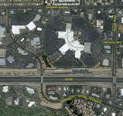
(Source: Google maps, USGS, Digital Globe, U.S. Farm Service Agency.)

Site Characteristics

The test site location experiences high traffic volumes due to access provided to the U.S. 60 freeway from communities to the north and the commercial shopping area anchored by the Superstition Springs Center mall. Both Power Road and Southern Avenue are six-lane arterials with a raised median with curb cuts for left turns at intersections and at major un-signalized entrances to the shopping mall. The City of Mesa primarily desires to provide access equity to and from the mall while at the same time providing a pipeline operation to and from U.S. 60 along Power road. The city’s installation of the ASCT was initially driven by the fluctuations of traffic during seasonal changes attributable to an increase in winter visitors to the region, the school calendar, and the mall.

As discussed in Chapters 5 and 6, some findings may be less compelling due to the limited project size. In particular, travel time runs are relatively short so some comparison results (e.g. buffer times) are amplified. In particular, this highlights the general conclusion of the project that the community should strive to minimize the use of percentages for reporting validation findings.

Location of Traffic Signals

There are eleven signalized intersections within the test site. The following five traffic signals were enabled for phase and detector data logging in this analysis:

1. Southern Avenue and Superstition Springs Boulevard.
2. Power Road and Southern Avenue.
3. Power Road and Hampton Road.
4. Power Road and U.S. 60.
5. Power Road and Superstition Springs Boulevard.

Figure 38 below shows the location of each of the traffic signals. Power Road and Southern Avenue and Power Road and the U.S. 60 interchange are the critical locations in the system. The signals where high-resolution phase and detector data were not collected are also operated in adaptive mode by the ASCT. An additional 10 intersections outside the study area are also operated by the ASCT but were not studied in this test.

Figure 38. Map. Test Site Traffic Signals.

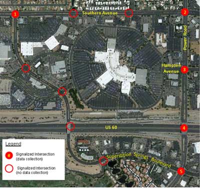
(Source: Google maps, USGS, Digital Globe, U.S. Farm Service Agency.)

Characteristics of Baseline Traffic Signal Operation

The existing City of Mesa coordinated traffic signal timing plans were used as a baseline comparison for the adaptive operation measures of effectiveness. There were three coordinated time-of-day timing patterns in operation. Table 2 below indicates the pattern schedule.

Table 9. Coordinated Timing Pattern Schedule.

Intersection(s)	Day	Start Time	End Time	Pattern
1 – Southern Ave and Superstition Springs Blvd	Monday-Friday	12 am 6:30 am 6:30 pm	6:30 am 6:30 pm 12 am	10 20 10
2 – Power Rd and Southern Ave 3 – Power Rd and Hampton Ave 4 – Power Rd and U.S. 60 5 – Power Rd and Superstition Springs Blvd	Monday- Friday	12 am 6:30 am 3 pm 6:30 pm	6:30 am 3 pm 6:30 pm 12 pm	10 20 30 10
1 – Southern Ave and Superstition Springs Blvd 2 – Power Rd and Southern Ave 3 – Power Rd and Hampton Ave 4 – Power Rd and U.S. 60 5 – Power Rd and Superstition Springs Blvd	Saturday	12 am 9:30 am 6 pm	9:30 am 6 pm 12 am	10 20 10
1 – Southern Ave and Superstition Springs Blvd 2 – Power Rd and Southern Ave 3 – Power Rd and Hampton Ave 4 – Power Rd and U.S. 60 5 – Power Rd and Superstition Springs Blvd	Sunday	All Day	All Day	10

For Intersection 1 at Southern Avenue and Superstition Springs Boulevard, the time-of-day timing includes an off-peak (night) and a peak (day) pattern schedule for weekdays and Saturday. The off-peak pattern is in operation all day on Sundays.

For the other four site intersections, Intersections 2 through 5, the time-of-day timing includes an off-peak, morning/mid-day peak, and afternoon peak pattern schedule for weekdays. The same off-peak and peak pattern schedule that Intersection 1 utilizes on Saturday and Sunday is also used for Intersections 2 through 5 on weekends. The other signals in the study area follow these patterns as well. Plans 10 and 20 utilize a 100 second cycle time and Plan 30 uses a 110 second cycle time.

Detection Layout

The City of Mesa uses a common phase and detector numbering scheme as shown in Figure 39. For example, phases 2 and 6 are always west and eastbound travel directions, respectively. Coordinated phases are varied by pattern if necessary. At all times of day and days of week in this test site, phases 4 and 8 are the coordinated phases on all intersections on Power Road. The ASCT used in this location uses only stop bar detection for adaptive operation. Each detector is 15 feet long and the trailing edge is four feet upstream of the stop bar. At Power Road and Southern Avenue, setback loops are also installed for collecting system detection data. These detectors are appropriate for computation of percent arrivals on green and platoon ratio. No other intersections in the study area have set back loops or detection zones.

Figure 39. Diagram. Detector Configuration and Phasing.

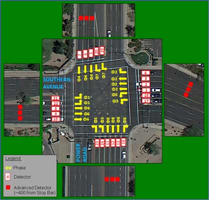
(Source: Kimley-Horn and Associates, Inc.)

Characteristics of Adaptive Traffic Signal Operation

The ASCT deployed in this location controls the durations by sending hold and force-off signals to the NEMA signal controllers over the SDLC bus. All cabinets are TS2. When adaptive control is running, the traffic controllers operate in FREE mode, so coordination is controlled by applying force-offs at the appropriate times. Phase sequence is not modified, but cycle time is allowed to vary at each intersection independently, every cycle. Cycles implemented by the adaptive system tend to hover around the configured coordinated cycle times. An example of the type of cycle variation implemented by the ASCT is provided in Figure 40. This figure illustrates a snapshot of a typical weekday. Similarly, splits are also varied on a cycle-by-cycle basis and tend to vary slightly around their default settings in the coordinated plan. This example shows the average splits for all eight phases implemented by the ASCT on Fridays during the main part of the day.

Figure 40. Line Graph. Example ASCT Cycle Adjustment Profile for Power and Southern.

(Source: Kimley-Horn and Associates, Inc.)

Figure 41. Line Graph. Example ASCT Split Adjustment Profile for Power and Southern (Fridays, 7 am-7 pm).

(Source: Kimley-Horn and Associates, Inc.)

Location of Bluetooth Detectors

Bluetooth travel time origin and destination detectors were placed at three intersection locations within the test site. Figure 42 shows the locations of the Bluetooth detectors. Each detector was paired with the other two to specify six unique routes:

• North and Southbound on Power Road from Southern to Superstition Springs (Pairs 1 and 2);
• East to Southbound, and North to Westbound from the Northwest corner to the Southeast corner of the system (upside-down “L” shape routes–Pairs 3 and 4); and
• East and Westbound on Southern from Superstition Springs to Power Road (Pairs 5 and 6).

Superstition Springs Boulevard intersects with both Power and Southern. This provides two alternative paths between the two locations at the northwest and southeast corners of the study area. It is not a particularly common route, as many 15-minute periods have no identified trips between the two locations. Based on qualitative analysis of the route travel time data, it is somewhat more common that drivers traverse southeast from Southern and Superstition Springs to Power and Superstition Springs (on either path) than vice versa.

Figure 42. Map. Bluetooth Detector Locations.

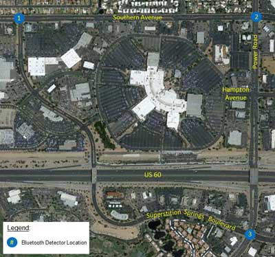
(Source: Google maps, USGS, Digital Globe, U.S. Farm Service Agency.)

Location of 24-Hour Tube Counters

Twenty-four-hour traffic volume counts were collected in four locations within the test site. The locations are described below and displayed in Figure 43. Both directions of travel were measured at each counter location.

1. Southern Avenue west of Power Road.
2. Southern Avenue east of Power Road.
3. Power Road south of Southern Avenue.
4. Power Road south of Superstition Springs Boulevard.

These volume counts were used to compare the route travel times with the level of traffic volume, and also to compare the throughput of the ASCT versus the coordinated operation. Traffic counter “C” is the critical location as it measures flows to and from the freeway.

Figure 43. Map. 24-Hour Tube Count Locations.

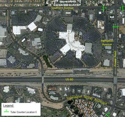
(Source: Google maps, USGS, Digital Globe, U.S. Farm Service Agency.)

The 24-hour traffic volume counts were collected over a period of 13 weeks from September to December 2012. No data were collected from October 23^rd through November 15^th. As is quite common in volume data collection studies that have significant duration, there were a variety of issues with the volume counts, ranging from destruction of the tube equipment due to street sweeping to unexplainable gaps in the data collection for one or more counters.

Probe Travel Time Routes

The Android GPS probe data collection tool was used to complete probe travel time runs using the floating car technique. Eight routes were traversed along Southern Avenue, Superstition Spring Boulevard, and Power Road. The routes are described below and shown in Figure 44.

1. Eastbound Southern Avenue from Superstition Springs Boulevard to Power Road.
2. Westbound Southern Avenue from Power Road to Superstition Springs Boulevard.
3. South-eastbound Superstition Springs Boulevard from Southern Avenue to Power Road.
4. North-westbound Superstition Springs Boulevard from Power Road to Southern Avenue.
5. Eastbound Southern Avenue to Southbound Power Road between Superstition Springs Boulevard intersections.
6. Northbound Power Road to Westbound Southern Avenue between Superstition Springs Boulevard intersections.
7. Southbound Power Road from Southern Avenue to Superstition Springs Boulevard.
8. Northbound Power Road from Superstition Springs Boulevard to Southern Avenue.

Figure 44. Map. Probe Travel Time Routes.

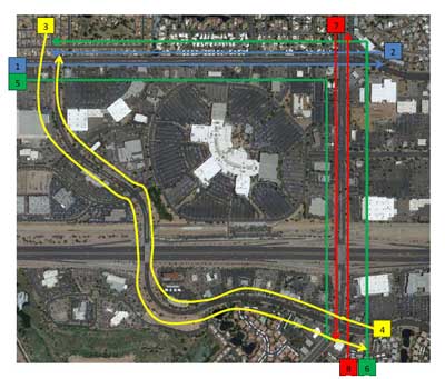
(Source: Google maps, USGS, Digital Globe, U.S. Farm Service Agency.)

The probe travel time runs were completed over a two week period. Table 10 displays the schedule for execution of the probe travel time runs. Data regarding approximately 24 travel time runs, three for each route, were collected for each two-hour peak period and during some off-peak times. Probe travel runs are quite expensive, which is one reason why the supplementary route travel times and high-resolution phase and detector data are critical to the analysis approach and a key recommendation resulting from this project. As stated earlier in the chapter, it is imperative that travel time runs start significantly upstream of the first intersection in the system and end after clearing the last intersection on the route.

Table 10. Probe Travel Time Schedule.

Day of the Week	Dates	Peak Period	Time
Tuesday	11/27, 12/4	Mid-Day PM	11 am – 1 pm, 4:30 pm – 6:30 pm
Thursday	11/29, 12/6	Mid-Day PM	11 am – 1 pm, 4:30 pm – 6:30 pm
Friday	11/30, 12/7	AM Mid-Day PM	6:30 am – 8:30 am 11 am – 1 pm, 4:30 pm – 6:30 pm
Saturday	12/1, 12/8	Mid-Day PM	11 am – 1 pm, 4:30 pm – 6:30 pm

Adaptive On/Off Schedule

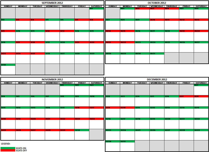
For the purpose of this study, the ASCT was turned on and off for randomized periods of time during the validation period. Figure 45 illustrates the days when the ASCT was in operation and when the coordinated timing plans were in operation from September 2012 through December 2012. On the days between 11/23 and 11/26 the ASCT failed due to hardware malfunction. The system is shown in adaptive mode for this period, but it was actually operating the intersections “FREE” at that time.

Figure 45. Calendar. ASCT On/Off Schedule.

(Source: Kimley-Horn and Associates, Inc.)

The ASCT was “ON” for the following:

• 8 Sundays
• 7 Mondays
• 8 Tuesdays
• 9 Wednesdays
• 9 Thursdays
• 7 Fridays
• 8 Saturdays

The ASCT was “OFF” for the following:

• 7 Sundays
• 8 Mondays
• 6 Tuesdays
• 5 Wednesdays
• 5 Thursdays
• 7 Fridays
• 7 Saturdays

Data Collection Discussion

A quality data collection process and validation of raw data are essential to reliable data analysis. This section discusses how the different types of data were collected and prepared for analysis. Figure 46 is a comprehensive schedule showing the data that were collected on each day during the study period. Each row of the schedule represents a different type of data. The top row indicates if the ASCT was ON (green) or OFF (red) on that given day. Data types that are highlighted in a solid color for their row were complete for that given day. Days with incomplete data are not highlighted and days with zero data have no text or color. Due to a variety of real-world hardware and software functionality challenges, as can be seen from the figure, the data are not comprehensive for all data types for the entire period. The Purple color in the ASCT ON/OFF row of the schedule indicate those days when the ASCT was supposed to be on but was failed free due to field equipment failure.

Figure 46. Schedule. Data Availability Over the Study Period.

(Source: Kimley-Horn and Associates, Inc.)

Measures of effectiveness were produced from the data collected and processed into reports using tools available in the validation system. In addition to applying the reporting tools developed for the project, the MOE data were also exported into a comprehensive Excel database and dynamically analyzed using pivot charts. Representative results are presented in Chapter 5.

Phase Timing Data

As discussed, in Chapter 3, raw phase timing and detector actuation data are continuously collected by the ASC/3 controllers operating the test site intersections. These raw binary phase timing data files are retrieved from the intersections using an FTP script and then run through a PHP script that converts the binary into CSV files. The CSV files were then parsed by the import process to the validation website and the MOEs computed. In many cases, as illustrated in Figure 19, missing and incomplete binary files confound the analysis process. Regardless, this source of detailed information from the field controllers is invaluable in reducing the cost of validation and performance measurement analysis. Improvements to these data storage processes on field controllers to improve the reliability or use of third-party devices in locations with obsolete controllers are critical to enhance state of the practice in MOE computation.

Bluetooth Travel Time Data

The Bluetooth travel time data was collected by the detectors and stored by the Bluetooth device vendor at the vendor’s website. The Bluetooth readers are connected to the city’s IP network. City IT staff allowed the Bluetooth devices to connect to the internet to transmit the vehicle match data for processing. The information was imported to the validation system using an automated download of the Bluetooth travel time data from the vendor website. Similar to some of the challenges of data collection from the field controllers and the tube counters, a variety of real-world issues confounded the collection of the Bluetooth travel times for the first month of the effort. Extending support to additional Bluetooth data collection vendor systems will improve state of the practice in MOE computation.

24-Hour Tube Count Data

The 24-hour tube count data was first reviewed manually to identify collection errors or inconsistencies. Data from several locations were damaged by street sweepers and recorded zero vehicles or a value significant amount less than expected. These invalid data values were removed from the data set and are not included in the analysis. The tube count volume data was summarized in 15 minute intervals and imported into the validation system via the import process. Missing data are marked in Figure 19 in brackets [] with the letter designation of the counter and NB, SB, EB, WB designations if the missing information is isolated to one direction or the other. AM or PM annotations are appended to the letter designation if the missing data are isolated to morning or evening.

Probe Travel Time Data

The probe travel time data are sent automatically via the Android GPS probe data collection app. Each run was reviewed manually to identify any data collection errors or runs where cellular coverage was intermittent. Minor errors such as route mislabeling by the data collectors were repaired manually in the database.