Operations Benefit/Cost Analysis Desk Reference

Chapter 5. Conducting B/C Analysis for Operations

Selecting the Appropriate Methodology/Factors Influencing the Analysis Approach

The process of selecting an appropriate method or tool for use in the B/C analysis is a critical step in ensuring the eventual success of the effort. As discussed in Chapter 4, there is a wide variety of existing tools available for conducting B/C analysis of TSM&O strategies. Likewise, there is often great opportunity for practitioners to develop their own customized analysis approach if the available tools do not meet the exact needs of their analysis. Often, these custom approaches are built by borrowing capabilities from existing tools; and enhancing the process with customized methods configured to available data, existing regional analysis tools, and the specific needs of the analysis.

Prior to initiating any analysis, practitioners are encouraged to carefully weigh the factors influencing the analysis approach. Careful assessment of the analysis needs and mapping to an appropriate analysis method or tool will provide for a better use of scarce analysis resources, and help minimize the possibility of discovering that the selected analysis method is incapable of successfully completing the analysis when the evaluation is half-finished.

The sections below present expanded discussion of multiple factors that should be considered in selecting a methodology and customizing an analysis approach. These factors include:

• Geographic scope;
• Types of strategies;
• Need for/purpose of study;
• Desired MOEs;
• Required level of confidence in results;
• Available tools and data;
• Available analysis resources; and
• Other factors.

Geographic Scope

The geographic scope of the strategy to be analyzed plays a key role in developing the analysis approach. Some TSM&O strategies may be deployed and influence only a limited geographic area, such as an intersection, a freeway interchange, or a single corridor. Other strategies may be deployed on multiple corridors or even regionwide (e.g., 511 traveler information systems). The scope of the deployment(s) to be analyzed is a critical factor in determining the appropriate facilities to include in the analysis, as well as a determinant in selecting an appropriate analysis tool.

Another issue to consider when assessing the geographic scope to capture in the analysis is the effect of transfers from other regions. For example, an economic analysis may indicate a regional increase in jobs as a result of the increased regional productivity provided by an improvement. This would be seen as a benefit for the region gaining the jobs, but might be a disbenefit for the region where the jobs moved. If the analyst were conducting an analysis of the benefits that could be gained if the improvement were funded from 100-percent local funding, they may include these benefits as they represent a regional gain. If, however, the analysis were being completed for an improvement that was anticipated to be funded through state or national sources, these benefits would represent a transfer and should not be included. At the national scale, interstate and interregional transfers should not be included – only the net change on a national scale should be considered.

Prior to developing the analysis approach, practitioners should carefully assess the possible impacts of the TSM&O strategy to be analyzed, and determine the likely geographic extents of the impacts to various regional facilities. It is important that the analysis be designed to fully capture not only the impacts at facilities immediately adjacent to the proposed deployment, but also capture broader network impacts due to likely traveler changes in route mode or time of travel. For example, an analysis of a ramp metering deployment should not only attempt to assess the change in roadway performance within the immediate merge area, but also should attempt to include an assessment of conditions in the ramp queue, at adjacent intersections, and possibly on parallel arterials or freeway facilities, if they are likely to be impacted by the deployment. Failure to include all the likely facilities and modes likely to be impact by a strategy risks understating or overstating the benefits of the strategy.

The anticipated geographic reach of impacts of a TSM&O strategy also plays a key role in the selection of an appropriate analysis method/tool. Different analysis methods and tools are typically more appropriately scaled to analysis at different geographic scopes. For example, analysis of a TSM&O strategy on a corridor level may be most appropriately assessed using a multiscenario simulation, model-based approach; however, if an assessment is required on a regionwide basis, the simulation approach may prove to be too resource demanding to be practical. Table 5-1 presents a general overview of the tool categories (presented in Chapter 4) and their appropriateness to various geographic scales. As a general rule, as shown in the table, increases in the complexity of the analysis methods typically results in a smaller appropriate geographic coverage, often due to the resources necessary to conduct a very robust analysis on a broad scale.

Table 5-1 Analysis Methods/Tools Mapped to Appropriate Geographic Scope

Analysis Method/Tool	Appropriate Geographic Scope
Sketch-Planning Methods	Isolated Location
	Corridor
	Subarea
	Regionwide (Dependent on the specific analysis tool selected)
Post-processing Methods	Corridor
	Subarea
	Regionwide (Assumes post-processing method is applied to the regional travel demand model)
Multiresolution/Multiscenario Methods	Corridor
	Subarea

In addition to helping determine the most appropriate tool category to apply, the intended geographic scope of the analysis may play a factor in identifying specific tools to be considered. For example, a multiresolution approach utilizing a simulation model may be proposed for a particular analysis; however, different simulation packages/platforms are available that can support analysis at different geographic scales. For example, macrosimulation models provide less detailed analysis, but can provide simulation over a wider regional scale. Mesoscopic simulation models provide more detailed analysis, but are often limited to a subregional geographic scale. Microsimulation models provide the most detailed analysis, but are often limited to analysis on a corridor scale, given the data and resource requirements necessary to develop these models. In designing the analysis, the practitioner must make decisions regarding the tradeoff between the detail available in the simulation model and the geographic coverage that will be possible, given the available resources for the analysis. Figure 5-1 provides an overview of the different types of simulation tools mapped to their typical geographic scales.

Figure 5-1. Different Simulation Analysis Tools are Appropriate to Different Geographic Scopes

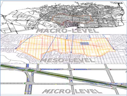
Source: FHWA Traffic Analysis Toolbox – Volume II, 2004.

In situations where a great amount of operational detail is required, but the analysis resources do not allow for full modeling or data collection on all the regional facilities impacted by the deployment, practitioners may want to consider the use of representative corridors for analysis. In this approach, one or more representative corridors are selected for detailed analysis, and the results are then extrapolated to other regional facilities. For example, in a well-known evaluation of the ramp metering system in the Minneapolis/St. Paul metropolitan region, the benefits of metering were examined regionwide; however, the analysis resources did not allow for detailed data collection and analysis on all individual corridors in the region. Instead, the analyst carefully selected four representative freeway corridors in the region: 1) a downtown corridor, 2) a radial corridor inside the beltway, 3) a radial corridor outside the beltway, and 4) a section of the beltway corridor. Figure 5-2 shows the selected representative corridors in relation to the overall regional transportation system in the Twin Cities.

Figure 5-2. Use of Representative Corridors in an Analysis

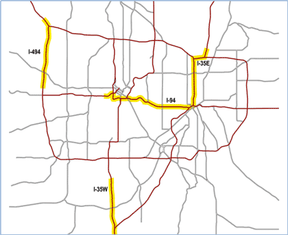
Source: Minnesota DOT Twin Cities Ramp Meter Evaluation, Final Report, 2001.

Detailed data collection and analysis were performed on the four representative corridors, and then the analysis results, in terms of percentage changes in key MOEs, were extrapolated to all other corridors in the region based on the type of the corridor being analyzed. Performing the analysis in this way allowed for the required detailed analysis of specific benefits, but also allowed for the regional compilation of total benefits within the resource requirements of the study.

Types of Strategies

The type of strategy, or combinations of strategies, to be analyzed and compared within the B/C analysis is a key factor in determining the analysis approach. At the most basic level, the analyst should first determine if the analysis would need to:

• Only evaluate and prioritize TSM&O strategies compared with each other;
• Compare TSM&O strategies alongside alternative scenarios with more traditional capacity enhancements; or
• Evaluate various alternative scenarios containing combinations of TSM&O and more traditional capacity enhancements.

A list of the strategies (TSM&O and traditional capacity projects) to be analyzed should be developed prior to the identification of the analysis approach. Many practitioners also find it useful to graphically map the strategies to be analyzed to individual analysis scenarios that will be analyzed. Figure 5-3 shows a sample mapping of strategies and scenarios that shows the breakout of strategies to be performed, as well as identifying those strategies that will combined and analyzed together. This display is useful in identifying analysis that needs to be conducted on more traditional capacity enhancements (shown at the “Alternative” level in Figure 5-3), as well as scenarios that include only TSM&O strategies and combinations of TSM&O and more traditional strategies (shown as the “TSM&O Options” in Figure 5-3). This preliminary identification of analysis scenarios also is useful in identifying the number of individual analyses that will need to be performed.

Figure 5-3. Mapping of Strategies to Analysis Scenarios

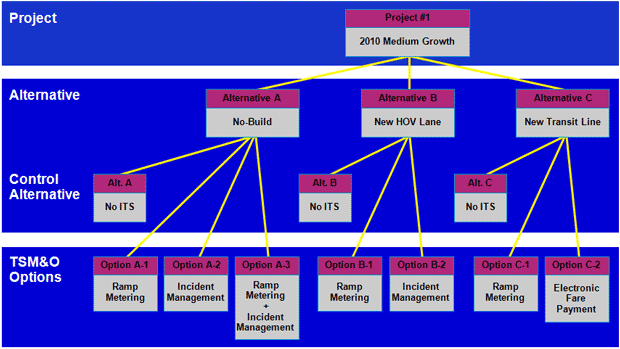
Source: FHWA IDAS Training Course Participant Workbook, 2010.

This list of alternative strategies/scenarios should then be assessed to project the likely impacts of the strategies, including:

• What are the MOEs that may be affected?
• What are the facilities that will likely be impacted?
• Which modes will be impacted?
• What are the likely traveler behavior changes (e.g., route change, mode shift, temporal shift, etc.)?
• What are the time periods that likely will be impacted (e.g., are the strategies intended to be operated all day or only during peak periods or special conditions)?
• Will the timing of the strategy’s implementation need to be considered (e.g., are all alternative strategies projected to be deployed on a similar time horizon or would the deployment of certain alternatives be delayed until future years [See discussions later in this Chapter on the Impacts of Selecting Different Time Horizons and the Impact of Time on Monetary Value]).

Answers to these questions will allow the analyst to begin formulating the analysis approach, including selecting an appropriate analysis tool(s), as well as identifying preliminary input data needs. The assessment of strategies to be analyzed should be weighed against the other factors presented in this section to formulate the final analysis approach.

Need for/Purpose of Study

As discussed in Chapter 2, B/C analysis can play a role across a wide range of transportation planning processes and phases. The need for the analysis (or the planning objective that the analysis is intended to fulfill) is a key factor to consider in developing the analysis approach, and often helps to determine:

• The required level of confidence in the accuracy of the results;
• The number of alternatives to be analyzed; and
• The appropriate level of resources needed to conduct the analysis.

In early planning phases, for example the preliminary screening of alternatives, there is often a need to quickly conduct high-level, order-of-magnitude analysis of a large number of alternative scenarios. This analysis would likely require an approach that could be quickly implemented and repeated for a number of scenarios; however, the level of detail in the analysis may not be as critical. Alternatively, at the other end of the planning spectrum during the final alternative prioritization and design process, there may be the need to conduct very detailed analysis of a small number of scenarios. This analysis may require a substantially different analysis approach than used for preliminary screening needs. Figure 5-4 provides a comparison of different analysis tools mapped to different phases of the planning process, as well as the level of detail provided by the different analysis tool types, developed for an FHWA workshop series on Applying Analysis Tools in Planning for Operations. The figure shows how the proposed analysis method and/or tool may be influenced by the need for detail related to different phases of the planning process.

Figure 5-4. Comparison of Analysis Methods with Various Stages of the Planning Process and Need for Analysis Sensitivity

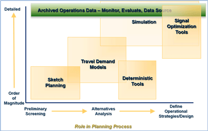
Source: FHWA Workshop Series – Applying Analysis Tools in Planning for Operations Participant Workbook, 2011.

Desired MOEs

Different TSM&O strategies often may have impacts on different MOEs. Likewise, different regions may place a higher priority on particular MOEs. For example, a region that is in noncompliance for a particular emissions category may have requirements that an assessment of that measure be included in all regional analysis. Therefore, the analyst should carefully consider the MOEs to be used in the analysis when setting up the approach and making decisions on applicable analysis tools.

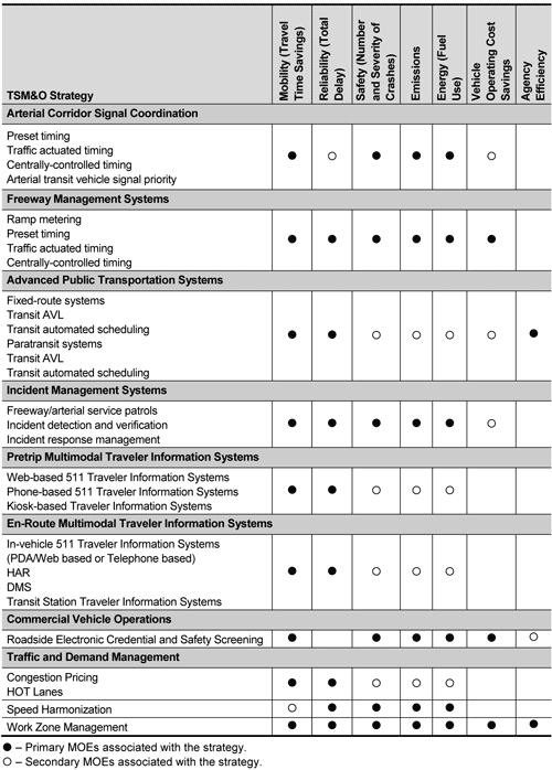
Figure 5-5 presents an overview of TSM&O strategies and their primary and secondary impacts on various MOEs.

In addition, Figure 4-7, presented earlier, shows the capabilities of a wide range of analysis tools in examining particular performance measures. In planning for the analysis, practitioners should:

• Carefully identify the MOEs likely to be impacted by the strategies and projects they want to evaluate;
• Prioritize the MOEs to the needs of the analysis and the individual needs of the agency; and
• Select a tool or analysis method that best supports the analysis of the prioritized MOEs.

Figure 5-5. TSM&O Strategies Mapped to Likely Impacts on MOEs

Required Level of Confidence in Results

The needs of different analyses often require different standards in terms of the level of confidence that is needed in the analysis outputs and results. Preliminary screening of projects may only require that order-of-magnitude results be generated to help categorize long lists of projects into high-, medium-, and low-priority levels. At the other end of the spectrum, very detailed and accurate results may be needed for finalizing design decisions or establishing strategy operating parameters. It is critical, therefore, that the level of confidence in the results required by the study needs be carefully considered in planning the analysis, and in selecting the appropriate analysis method/tool.

The required level of confidence in the results of the analysis often has a direct influence on the analysis resources that will be required. Typically, analysis requiring highly detailed and accurate results will demand the application of more robust analysis methods and tools that may necessitate a greater application of resources, including analysis budget, schedule, computing resources, and staff expertise. The tradeoffs between the required level of confidence and the level of resources need to be carefully weighed in order to avoid selecting an inappropriate analysis method. Inappropriate analysis methods can include both:

• “Underpowered” tools or methods that are not sufficiently robust to produce results with the desired level of confidence; and
• “Overpowered” tools or methods are overly detailed for the analysis need and may end up requiring more analysis resources than are available for the study.

Either of these above situations has the potential to negatively impact the integrity of the analysis and may result in the analysis being scrapped and started over using a more appropriately scaled tool or method, often at great cost.

While the level of confidence in the results is largely a product of the analysis tool or method selected, it is also related to the amount of effort put into customizing, calibrating, and validating the various tools. For very simple analysis requiring order-of-magnitude detail, practitioners may choose to simply apply parameters, impact measures, and benefit values based on national averages. As the need for greater confidence in the level of accuracy increases, practitioners will want to place greater effort on identifying and applying customized analysis parameters within the selected method/tool that more closely match the local experience and traffic conditions.

The level of confidence required for any individual analysis is determined individually for each analysis based on a number of factors, including:

1. The role fulfilled by the analysis in the planning process;
2. The intended audience for the analysis results;
3. The number of alternatives to be evaluated;
4. The availability and accuracy of underlying data and models; and
5. Subsequent analysis to be performed based on the analysis results.

Among these factors, the role that the analysis fulfills in the planning process often has the most substantial influence on the level of confidence and detail required. Figure 5-4, shown earlier in this section, showed that activities occurring earlier in the planning process, such as preliminary screening of alternatives, often require a lower level of detailed results, and confidence in the results, while activities occurring during later stages of the planning process, such as final prioritization of alternatives or design work, may require highly detailed results that also require a high degree of confidence in the accuracy of the results. As shown in Figure 5-4, the need for detail and accuracy often drives decisions regarding the appropriateness of different tools and methods.

The level of confidence required in the analysis results is often the most substantial factor determining the analysis approach and the level of analysis resources that will be required to meet these needs. The following section provides additional discussion on the need to balance the analysis needs with the available resources.

Available Analysis Resources

Ideally, every B/C analysis would be conducted with the highest level of detail and rigor to provide:

• Comprehensive analysis of all the MOEs possibly impacted by the selected strategy;
• Analysis on a wide geographic scale to ensure the full capture of all regional benefits; and
• The highest level of confidence and detail of the analysis approach.

The reality of constrained budgets available for analysis, however, means that practitioners must often weigh the actual needs of the analysis against the available resources to balance the needs against the ability to support those needs.

Different analysis methods and tools often require substantially different levels of resources in order to successfully complete the analysis. The resources required for an analysis may include:

1. Budget resources;
2. Schedule;
3. Staff knowledge and expertise;
4. Computing resources;
5. Knowledge and data on local traffic conditions and operations;
6. Data availability and collection capabilities; and
7. Time and costs of utilizing supporting tools, models and analysis.

Some simple sketch-planning tools are designed to be applied at a low cost on a quick-timeframe basis. Utilizing the basic default parameters available in many of these tools, along with readily available data, a novice analyst could produce a basic B/C analysis in an afternoon. On the other hand, many analyses involving highly robust multiresolution/multiscenario methods may require six months to a year to complete at a cost of hundreds of thousands of dollars. Table 5-2 presents an overview of the general categories of analysis methods and tools compared with their approximate relative costs. Dollar budget costs presented in the table are approximate and represent the staff time required to complete an analysis (or the equivalent cost of a consultant).

Table 5-2 Analysis Tools and Methods Mapped to their General Resource Requirements
(Estimates are provided for a “typical” analysis. Actual time and budget resources would be dependent on the number of alternatives, geographic scope, and effort required to compile the appropriate input data)

Method/Tool	Resources Required
Sketch planning	Budget – Low ($1K to $25K)
	Schedule – 1 week to 8 weeks
	Staff Expertise – Medium
	Data Availability – Low
Post-processing methods	Budget – Medium/High ($5,000 to $50,000)
	Schedule – 2 months to 1-year
	Staff Expertise – Medium/High
	Data Availability – Medium
Multiresolution/multiscenario	Budget – High ($50,000 to $1.5 million)
	Schedule – 3-months to 1.5-years
	Staff Expertise – High
	Data Availability – High

Available analysis resources should be identified early in the analysis planning process, along with the other factors discussed in this section. The analysts and their managers should then carefully weigh the needs of the analysis with the projected costs. The estimate of resources should also consider the contingency costs of conducting any additional analysis, or evaluating new alternatives that may arise during the project prioritization process. If, during this assessment, the project needs and the available resources are found to not be aligned, then the analysts and their managers need to seek a balanced resolution, but either cutting scope and/or requirements from the analysis (e.g., lessening the number of alternatives to be analyzed or reducing the complexity of the analysis); or by increasing the available resources to meet the needs of the analysis. Failure to do so will result in either a cost overrun, a poorly conducted analysis that does not meet its original intent, or both.

The TOPS-BC application, developed in parallel with this Desk Reference, provides a decision-support tool to aid practitioners in weighing the needs of the analysis with the resources that may be required. Additionally, the FHWA initiative on the Traffic Analysis Toolbox also provides guidance on the level of resources needed to perform different types of analysis (using different types of analysis tools). (FHWA Traffic Analysis Toolbox – Volume II, 2004.)

Other Factors

The factors presented above often comprise the most critical determinants in identifying and planning a successful analysis approach. As discussed, there is often the need to carefully balance the tradeoffs between the various factors (e.g., more robust analysis often requires additional resources to complete) in the final selection of an appropriate analysis approach.

In addition to these factors, several additional aspects of the analysis should be considered during the early planning and scoping effort in order to effectively establish a suitable analysis approach. These additional factors include:

• Established B/C analysis procedures and framework – Many regions and agencies have long used B/C analysis for assessing and prioritizing various transportation projects. This long-term use has often resulted in procedures, benefit valuations, and analysis frameworks being established. These established guidelines should be followed to the degree possible in order to remain consistent with the local planning process. If the established procedure has primarily been used to conduct B/C analysis of more traditional capacity-enhancing projects, some modification of the framework may be necessary to make it appropriately sensitive to the needs of MOEs used for analysis of TSM&O strategies. See Chapter 4 for an expanded discussion of these issues.
• Available data to support the analysis – In regions with rich sources of available data, such as a region equipped with a robust and reliable archived data system, some more advanced analysis methods may be pursued at substantially less cost than could be considered in other more “data poor” regions. The readily available data in the robust data region could be tapped to support more advanced analysis methods and tools than in the data poor region, where substantial resources may need to be applied to manual data collection efforts in order to establish the baseline dataset necessary to support the analysis effort, or calibrate and validate the needed analysis tools.
• Available tools to support the analysis – Many analysis tools commonly used to provide input data for B/C analyses were originally developed for other purposes. For example, if a detailed simulation model has been previously developed, calibrated, and validated for a regional corridor, a more advanced and detailed analysis method may be possible at a substantially lower cost than would be possible in a corridor, where an existing model did not exist. All existing and underdevelopment tools that may be available to support an analysis should be inventoried during the analysis planning phase, along with the data outputs available and the level of effort required to conduct analysis using the tool, and weighed along with the other critical factors in identifying the optimal analysis approach.

Determining the Appropriate Timeframe to Use

As opposed to many standard transportation analyses that examine the system performance related to a particular improvement alternative for a specific analysis year (e.g., current year 2011 baseline analysis, or future year 2030 analysis), many B/C analysis attempt to capture the comprehensive benefits that flow as a result of an improvement over the life cycle of the deployment or other another selected time stream (e.g., 10-, 20-, or 30-year time horizons). The purpose of this approach is to spread out both the benefits and costs over an appropriate timeframe to allow for a meaningful analysis. For example, a practitioner would not want to compare the total costs for a strategy with a single-year estimate of benefits.

Therefore, the selection of an appropriate timeframe or time horizon to use in the analysis can take on more importance than in other transportation analyses. The implications of selecting and using different timeframes for analysis are discussed in the following sections.

Impacts of Selecting Different Time Horizons

The practice of capturing benefits and costs over a defined time horizon in transportation-related analyses is common and is largely tied to the analysis of large-scale infrastructure projects, where a general useful life of the project is well known. For example, the costs (capital implementation costs plus continuing operations and maintenance costs) of a new bridge or roadway could historically be relatively well estimated over the expected life (e.g., 30 years) of the infrastructure or pavement. The benefits often were relatively static over the analysis timeline as well, providing for an easy calculation and comparison of benefits and costs over the selected timeframe.

Applying this same traditional timeframe approach to TSM&O strategies can add complexity to the analysis due to the following factors:

• Benefits of TSM&O strategies can be extremely variable – For example, a TSM&O weather management system would be expected to have varying benefits year after year, depending on the number of inclement weather days. This differs from more traditional capacity improvements that would be expected to have nearly the identical benefits year after year.
• TSM&O strategies often have shorter useful life of equipment and require more frequent replacement cycles – Many major infrastructure projects, like adding a lane to a regional freeway facility, have a relatively long and predictable useful life (e.g., 20 to more than 30 years) before requiring complete replacement. Many TSM&O strategies, on the other hand, are technology based and some key components may need replacement on much faster cycles (e.g., every 2 to 5 years). As a result, it is more difficult to place an overall “useful life” on TSM&O strategies since they have equipment with much shorter useful lives, yet are often also assumed to be operated in perpetuity once they are deployed.
• Costs of technology are changing over time – Many TSM&O strategies rely heavily on emerging technology; and as the economies of scale of new strategies expand, the costs often decrease. Therefore, evaluating a pilot project based on the initial development and implementation costs may not be accurate, as the costs could be expected to decline significantly in future years as a result of technology improvements.

These factors, combined with the effects of inflation and the time value of money, which impact all B/C analyses performed over a time horizon (discussed in a subsequent section), make selecting a time horizon for the analysis a critical effort that potentially impacts the results.

Many agencies maintain their own procedures for conducting B/C analysis that specify the length of the analysis period that should be applied. This standard should be applied whenever consistency with the established B/C framework is required. Likewise, if a B/C analysis is required to fulfill part of a funding request, the funding mechanism may specify a specific time horizon be used. For example, the recent U.S. DOT TIGER Grant application process required that a 20-year time horizon be used in the B/C analysis. The analyst should research any existing agency practices and/or the specifications of any funding application prior to initiating the analysis to identify any requirements for a specific time horizon.

If no predetermined time horizon exists, the analyst may choose between several options for the time horizon for the analysis. If a stream of cost analysis is desired, the time horizon generally is scheduled to start with the first project expenditures, and extends through the useful life of the project or its most long-lived alternative, or some future time at which meaningful estimates of effects are no longer possible. (Transportation Benefit-Cost Analysis.)

If the time horizon selected is shorter than the expected life of one of the analyzed projects, and/or a project will need to be redeployed within the time horizon, the analysis may need to consider the salvage value or residual value of the equipment or deployment that remains at the end of the time horizon. For example, if a 20-year time horizon is selected for a light-rail project, it is likely that the rail vehicles and rail infrastructure will still have substantial remaining useful life at the end of the analysis period. In this situation, the residual value of this remaining life would need to be determined and added back into the analysis. Residual or salvage values are often used less in analysis of TSM&O strategies as the faster equipment replacement cycles lessen the salvage value for many of technologies and equipment.

An alternative option to using an analysis with a set time horizon is to utilize a single estimate of average annual benefits and costs. This measure is most typically used in analysis that seeks to compare and prioritize various TSM&O strategies with each other. TSM&O strategies are often well suited for analysis using average annual benefits and costs since they have relatively short life cycles, and are anticipated to be repeatedly redeployed in future years. Use of average annual benefits is also useful if only a single-year snapshot view of performance is available for the analysis (e.g., only a single forecast year of data is available for analysis).

Many current B/C analysis tools use average annual benefits and costs in their analyses, including the IDAS tool and the TOPS-BC tool that supports this Desk Reference. (TOPS-BC is capable of estimating average annual benefits and costs, or projecting the benefits and costs to a stream of costs that may be used with a time horizon selected by the user.) Average annual benefits are generally estimated based on a single forecast year, and are anticipated to be identical for all years. Average annual costs are estimated based on the capital cost of a piece of equipment divided by the anticipated useful life of the equipment. To this capital cost, an estimate of annual O&M cost is added to estimate the total average annual costs. For example, if a camera to be used in traffic surveillance strategy has:

• A total capital cost of $10,000;
• An anticipated useful life of 10 years; and
• Annual O&M costs of $2,000 per year, the average annual costs would be:

Average Annual Cost = ($10,000 capital/10 years) + $2,000 O&M = $3,000 per year

Impacts of Time on Monetary Value (Inflation and Discount Rate)

Two competing influences on future dollar values need to be considered in B/C analysis: inflation and discounting.

1. Inflation is the increase in prices for goods and services over time. It implies a loss in the value of money over time, as it erodes the purchasing power of a currency. Benefit/cost analysis for public-sector projects generally controls for inflation, using estimates of future costs and benefits that are expressed in terms of today’s (or some base year’s) prices. These are referred to as “constant” or “real” dollars. Consistent with this approach, the discount rate used in benefit/cost analysis represents the time value of money after adjustment for inflation. (Transportation Benefit-Cost Analysis.)
2. The Discount Rate is the recognition that a dollar today is worth more than a dollar five years from now, even if there is no inflation because today’s dollar can be used productively in the ensuing five years, yielding a value greater than the initial dollar. Future benefits and costs are discounted to reflect this fact.

Benefit/cost analyses typically ignore inflation because the prediction of future prices introduces unnecessary uncertainty into the analysis. Therefore, discount rates are typically based on interest rates for borrowing with the inflation component removed, yielding the “real” interest rate. This rate is typically calculated by subtracting the rate of inflation (consumer price index) from the interest rate of an investment, such as a 10-year U.S. Treasury bill. For example, if the interest on a 10-Year Treasury bill is 5.5 percent and the inflation rate is 3 percent, then the discount rate would be 2.5 percent. (Transportation Benefit-Cost Analysis.)

The discount rate for most projects in based on guidance provided by the U.S. Office of Management and Budget (OMB). The rate to be applied is related to the type of the project and the expected benefits and costs. If the project is anticipated to have benefits to the general public (societal benefits such as travel time savings or crash reductions), the OMB currently suggests a discount rate of 7 percent, which represents the real discount rate on private investment. If, however, the analysis includes benefits and costs exclusively related to the public agency, for example, an analysis of an investment that would bring about a cost savings to the agency, the OMB suggests using the real discount rate for public-sector investments, which is often lower due to the lower risk associated with government borrowing. The OMB publishes “real” interest rates on its web site. Table 5-3 presents the real rates published on the site in July 2011. Generally, if there is a mix of societal and agency benefits within the same analysis, only the private-sector investment discount rate (7 percent) is used.

Table 5-3 Real Discount Rates 2011 (Public Investment)
(in Percentage)

Time Period	3-Year	5-Year	7-Year	10-Year	20-Year	30-Year
Discount Rate (%)	0.0	0.4	0.8	1.3	2.1	2.3

Source: White House Office of Management and Budget, 2011.

Real discount rates, as shown in Table 5-3, represent rates in which inflation has been removed. These real rates are to be used in B/C analysis for discounting real (constant-dollar) flows.

Available Resources for Identifying the Benefits of Operations Strategies

Often, one of the most challenging aspects of conducting B/C analysis of TSM&O strategies is identifying the likely impact or benefit of the strategy. This is particularly true for emerging technologies or strategies, where few real-world deployments exist to provide empirical evidence on the likely impacts to various MOEs. Several options for researching the likely benefit levels that may be used in an analysis are discussed in this section.

The TOPS-BC application that supports this Desk Reference maintains a look-up database of likely impacts of various TSM&O strategies related to several MOEs. Figure 5-6 shows a view of the navigation screen for this capability in TOPS-BC. To research likely impact levels of TSM&O strategies, the user would select a “Strategy” and “Impact Category” from the pull-down menus. Based on this input, TOPS-BC would display a “Typical Range of Expected Impacts,” assuming there is sufficient data to formulate a range for the selected strategy and impact category.

Figure 5-6. Sample View of TOPS-BC TSM&O Impact Look-up Function

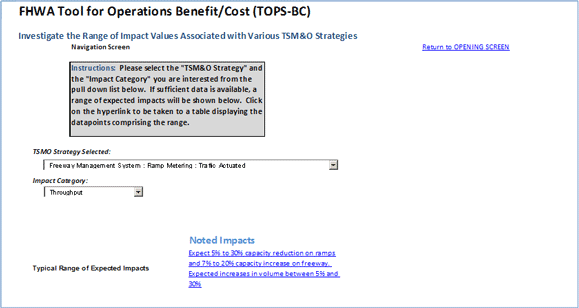
Source: FHWA TOPS-BC model.

The range of expected impacts is based on a compilation of evaluations and studies that have gathered empirical evidence on the impact of these strategies in national and international locations. This range also often considers the predicted impacts used in various traffic and B/C analysis tools as the default impacts used in the calculation of benefits for the strategy, when available. The user may view these individual studies and model data on subsequent worksheets in the TOPS-BC application. Descriptions of the observed impacts are brief, but links are provided to the source documentation so the user may research further any interesting information.

Another valuable resource for researching the potential benefits of TSM&O strategies is the ITS Benefit Database maintained by U.S. DOT Research and Innovative Technology Administration’s (RITA) ITS Joint Program Office. The database allows users to research benefits information by strategy area, provides a rich resource for identifying benefits, and maintains a robust library of studies documenting the benefits of many TSM&O strategies. Figure 5-7 presents a view of the navigation page for the database site.

Figure 5-7. Sample View of U.S. DOT ITS Benefits Database Web Site

Configuring B/C Analysis to Local Conditions

As discussed in Chapter 3, many existing B/C tools and analysis frameworks maintain default parameters representing the anticipated impact to various MOEs. These are often based on national averages of observed benefits gathered from empirical studies in the case of widely available tools. For analysis frameworks that were developed for a specific region, these parameters may be more individually customized for that specific region. For simple analysis, for example, a quick, first-cut screening of alternatives, analysts may choose to use one of these widely available tools or perhaps a framework that was developed for another agency or region, and apply the method locally with little or no changes to these default settings. As the level of required confidence in the analysis results increases, however, users should increasingly place greater scrutiny on the default parameters, and modify these inputs accordingly to better configure the analysis to local conditions.

Ideally, analysts will be able to identify and obtain data specific to the local region that may be applicable in supplementing or replacing the default analysis parameters based on national averages. This data may be obtained from previously conducted evaluations that were conducted in the region, review and analysis of archived data, or other local sources. For example, in the Cincinnati analysis case study presented in Chapter 2, the OKI region analysts started the analysis with a thorough review of the analysis defaults. The defaults were scrutinized to assess if they were appropriate to the way the region operated its TSM&O strategies, and to identify any local sources of information that would be more appropriate. The analysts were able to identify a locally conducted evaluation of the reduction in incident duration caused by their FSPs, which they were able to use to replace the default parameter in the analysis. Likewise, some local survey results were used to refine the default amount of time saved by travelers as a result of DMS-provided information. These modifications substantially improved the overall analysis; in that, the parameters were better configured to local conditions. This configuration was performed for the local system costs and benefit valuation figures as well.

Where data is not available specifically representing conditions in the local area, the reference resources discussed in Chapter 5 may be used to assess the appropriateness of the default parameters and make adjustments to better configure the results to the local conditions. For example, an analyst working for a mid-sized region located in Midwest may want to review the individual studies highlighted in the TOPS-BC and the ITS JPO ITS Benefit Database to find individual studies conducted in similarly sized and located regions. If the results from these individual studies differ substantially from the national average default parameters, they may want to modify the parameters to be more representative of conditions in their region.

Finally, for more detailed multiscenario analysis, where the analysts may be attempting to individually model different scenarios representing various nonrecurring conditions, a preanalysis of existing conditions and the frequency of various nonrecurring factors may be warranted to develop meaningful analysis scenarios representing likely conditions. Robust data from archived data systems is often the best source for conducting this analysis for scenario development and identification. Table 5-4 presents an output of an analysis performed for the ICM Pioneer Site study conducted in Dallas. The analysis shows the frequency of occurrence of several factors related to congestion levels, and was used to identify likely analysis scenarios that most accurately represented the nonrecurring traffic conditions on the U.S. 75 corridor. By basing the test scenarios on the actual observed distribution of conditions, the analysis was better configured to local conditions.

Table 5-4 Distribution of Operating Conditions in U.S. 75 Dallas

Demand	Incident	Inclement Weather	Number of Hours	Percent
Med	No	No	247	33.9%
Low	No	No	136	18.7%
High	No	No	134	18.4%
Med	Minor	No	79	10.8%
High	Minor	No	55	7.5%
Low	Minor	No	55	7.5%
Low	No	Yes	9	1.2%
Med	No	Yes	5	0.7%
Med	Major	No	4	0.5%
Low	Major	No	2	0.3%
Low	Minor	Yes	2	0.3%
High	Major	No	1	0.1%
Med	Minor	Yes	0	0.0%
High	No	Yes	0	0.0%
High	Minor	Yes	0	0.0%
High	Major	Yes	0	0.0%
Med	Major	Yes	0	0.0%
Low	Major	Yes	0	0.0%

Source: ICM System – Analysis, Modeling, and Simulation Guide, Draft Final Report, 2011.

Estimating the Impacts (User and Societal Benefits) of the Operations Strategy

Estimating the benefits of various TSM&O strategies is tied to the type of project being evaluated. As detailed in Chapter 3, TSM&O strategies are often categorized into three groups:

1. Physical operations strategies – These strategies involve the deployment of physical infrastructure to the roadside or transit assets, and are intended to provide direct impact on transportation system performance through their operation. These strategies are often highly visible to the traveling public, and include a wide range of deployments, such as traffic signal coordination, freeway service patrols, 511 traveler information systems, HOT lanes, and DMS, among many others.
2. Supporting infrastructure – Supporting infrastructure includes those backbone capabilities that serve to support and enhance the functioning of the roadside Operations strategies. This backbone infrastructure includes items, such as traffic detection and surveillance, communications, and traffic management centers. Often, by themselves, these strategies have no direct intrinsic benefits. The benefits derived from these strategies are the improved performance of the roadside Operations strategies enabled by their deployment. For example, a traffic surveillance camera by itself has little direct benefit. The benefit is derived from the manner in which the information is use (e.g., when the surveillance from the camera is used by operators to implement different signal timing patterns, or detect and respond to an incident faster). Therefore, the measure of benefit of these supporting infrastructure components is often measured by estimating the improved efficiency of the roadside components supported by the backbone infrastructure, rather than attempting to directly estimate the benefits of the supporting infrastructure itself.
3. Nonphysical strategies – These strategies represent items intended to improve the efficiency and effectiveness of the TSM&O systems; and includes strategies, such as improved interagency coordination, the development of advanced operational plans (e.g., evacuation plans), or system integration. While there certainly can be benefits of these activities and there are often costs, there typically is little or no new physical equipment or roadside components. Similar to the supporting deployments, the benefits derived from these strategies are typically estimated by assessing the improvement in effectiveness of the existing roadside components provided by the strategy or activity.

Methods for estimating the benefits of these types of strategies are discussed in the subsequent sections.

Estimating the Impacts of Physical Operations Strategies

Most of the physical operations strategies impact one or more of the common MOEs. Previously presented, Table 5-5 shows the primary and secondary MOEs impacted by the strategies. Primary measures are those most closely correlated to the strategy, while the secondary measures may be more trivially impacted by the strategy, or may only be impacted depending on how the particular strategy is implemented and operated.

The goal in evaluating these types of strategies is to isolate the incremental change in the MOEs related to the deployment. In a real-world B/C evaluation of an existing strategy, empirical data representing conditions without the strategy (before deployment) is compared to data representing conditions with the strategy (after deployment) to assess the incremental change.

In a forecasting study, the “with” and “without” conditions are estimated using models or other predictive approaches to assess a baseline (without strategy) and an alternative (with strategy) scenario. The difference between the scenarios’ performance represents the incremental change due to the implementation of the strategy. In using modeled data for TSM&O strategies, it is important that the period of analysis in the model closely approximates the temporal (e.g., time-of-day) operating parameters of the strategy. For example, in evaluating a HOT lane strategy that is only anticipated to be operational during peak periods, the model used should represent the peak period, as this is the only time that benefits would be generated by the strategy. Use of a daily model in this situation could result in the overstatement of benefits, as benefits would be estimated to be falsely accruing to the strategy during off-peak periods, where it would not be expected to be operational.

The real-world before and after data or the modeled baseline and alternative scenario data are often entered into a spreadsheet or entered into an existing B/C analysis tool to provide a framework for calculating and documenting the change in the various MOEs. If the data used in assessing the incremental change represents a daily or portion of a day analysis (e.g., three-hour peak-period analysis), the resulting incremental change in the MOE needs to be annualized by applying a factor representing how many of those periods would be expected in a given year. Similar to selecting the appropriate time period for the analysis, it is critical that the analyst selects an annualization factor that accurately represents the operating parameters of the TSM&O strategy. For example, if the strategy were only operated on nonholiday weekdays, an annualization factor of 250 would be used to factor daily changes in MOEs to annual measures. For other strategies that are only operated during special events or other nonrecurring conditions, the annualization factor may be even less. Figure 5-8 shows a sample calculation of the daily change in various MOEs and the application of an annualization factor (250) to estimate the annual incremental change.

Figure 5-8. Example Calculations of Incremental Change MOEs

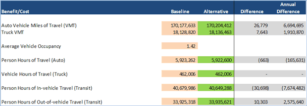
Source: San Francisco Bay Area MTC 2035 Long-Range Transportation Plan Project Performance Analysis, 2011.

The example shown in Figure 5-8 represents a relatively simple analysis, where a single-year forecast (2035 in this example) is used to represent the likely change in MOEs for all years. This assumes that the impacts and benefits of the deployed strategies remain fairly constant throughout the time horizon of the analysis. These incremental changes in MOEs may be expected to vary significantly, however, if the baseline (without the strategy) traffic conditions are expected to vary in future years. Depending on the underlying traffic conditions and the strategy selected, the benefits of the strategy could be expected to increase in future years – providing greater benefits as congestion increases – or decrease in future years – if the strategies incremental benefits are overwhelmed by increasing congestion.

Depending on the level of detail required by the analysis and the extent in which future conditions are expected to vary during the timeframe of the analysis, it may be necessary to add an analysis of one or more additional forecast years, and then interpolate the incremental change in MOEs between the analysis years to more fully capture these changing benefits.

For many typical MOEs (e.g., person hours of travel), the modeling method used as the source of the data (e.g., travel demand model, HCM analysis or simulation models) will be able to directly export the metric. Other MOEs, such as the number of crashes or amount of pollutant emissions, may be able to be directly estimated within the model structure (depending on the robustness of the regional modeling structure); or if not, may need to be assessed in a post-processing step. For example, many of the existing B/C analysis tools maintain the ability to estimate crashes and emissions based on simple outputs from the regional travel demand model.

For some of the emerging MOEs, such as travel time reliability, it is often necessary to employ a separate analysis method or structure (e.g., multiresolution- or multiscenario-based methods) to accurately assess these benefits as these measures are typically not yet well integrated with many regional modeling frameworks. See Chapter 5 for an expanding discussion of the methods that may be used to meet the challenges of assessing nonrecurring conditions in the analysis of TSM&O strategies.

Once the desired MOEs have been estimated and assembled in the B/C analysis tool or customized framework, appropriate benefit valuations (discussed in a subsequent section) are applied on a per unit basis (e.g., per hour of travel time saved, per number of injury crashes reduce, per ton of emissions reduced) to estimate the monetized user or societal benefit generated by the incremental change in the MOE.

Estimating the Impacts of Supporting Infrastructure

Estimating the impacts of supporting infrastructure, such as traffic surveillance and detection systems, traffic management centers, or communications systems, is often not as straightforward as estimating the benefits related to a physical operations strategy. Many of these supporting infrastructure projects have no inherent benefits associated with them. The benefits of these strategies flow from their ability to improve the physical roadside operations strategies. For example, the deployment of a camera surveillance system by itself would not be anticipated to generate any incremental changes to the typical MOEs (e.g., travel time, safety, vehicle operating costs, etc.). The benefit of the camera surveillance would be the impact of the additional data on improving other physical operations strategies – the camera images could be used to enhance the incident detection and verification procedures of the incident management program, or used to monitor an arterial in order to select appropriate signal timing strategies. Thus, the benefit does not accrue simply from deploying the supporting infrastructure, but from the improvement in operations of the physical roadside strategies which it supports.

To estimate the impacts of supporting infrastructure, the analyst first needs to map the supporting infrastructure to the roadside physical strategies it supports. An assessment then needs to be made regarding the influence of the supporting infrastructure. This assessment should evaluate:

• The degree to which the roadside physical strategy is influenced or enabled by the supporting infrastructure;
• Which specific MOEs will be impacted by the improved operation of the roadside physical strategy;
• The expected amount of time that the supporting infrastructure will be used to enable the roadside strategy (e.g., on a day-to-day basis, or only during infrequent occasions); and
• The proportion of cost of the supporting infrastructure that should be reasonably allocated to operating the roadside component (for example, if a camera surveillance system is anticipated to equally support an incident management program and the corridor traffic signal coordination strategy, the cost of the cameras should be proportionately allocated to both roadside strategies).

Based on this assessment, the anticipated impact for the roadside physical strategy should be increased to a higher point in the expected range of impacts for those MOEs anticipated to be improved by the enhancement provided by the supporting infrastructure.

If the supporting infrastructure and the roadside physical operations strategy are deployed in parallel as part of an integrated system, the costs used in the B/C analysis should include the full cost of the physical operations strategy and the proportion of the supporting infrastructure that can be reasonably allocated to supporting the specific roadside component. If, however, the supporting infrastructure serves to enhance an existing roadside strategy, the costs of that strategy should not be included in the analysis since they were paid for as part of another project. In these situations, only the cost of the supporting infrastructure that can be allocated to the enhancement of roadside component, and possibly any additional minor costs necessary to integrate the supporting infrastructure and the legacy roadside strategy should be considered.

Estimating the Impacts of Nonphysical Operations Strategies

Nonphysical strategies are intended to improve the efficiency and effectiveness of the deployed TSM&O systems, and involve their own challenges in assessment in a B/C analysis framework. The following represent some of the common nonphysical operations strategies, along with a description of an analysis approach.

1. System integration – Involves the integration of two or more systems to allow for the improved exchange of data between the systems and/or the coordinated operation of the systems. For example, a traffic signal coordination system could be integrated with a traffic incident management system to provide additional capacity on parallel diversion routes when incidents occur on a freeway facility. Similar to the analysis of supporting infrastructure deployments, analysts evaluating system integration strategies must carefully assess how and the degree which existing capabilities of the strategies to be integrated will be enhanced by the improved data availability or coordinated operations. The benefits would be estimated by modifying the expected impact on various MOEs to a higher level in the range of anticipated impacts to reflect this improvement.
   If the system integration involves the linkage of two or more existing legacy systems, the baseline scenario becomes the analysis of the physical operations strategies operated at their previous, nonintegrated impact level, and the alternative scenario would be the operations strategies operated at their enhanced impact level. The incremental benefit would be represented by the difference between these two scenarios. It is important if existing deployments are included in the analysis that the analyst not include the benefits already accruing due to the legacy components, but only include the incremental benefits of the enhanced operations due to integration.
2. Interagency coordination – Involves the exchange of information and/or agreements, allowing for the joint operation of various strategies across different agencies or jurisdictions. Similar to the approach for assessing system integration, the analyst and system operators will need to conduct an assessment of how and the degree to which the interagency coordination will improve existing or proposed physical operations strategies. An alternative analysis scenario should then be developed that increases the likely impacts on selected performance measures higher in the range of likely values. This alternative should then be run through the analysis process to estimate the change in MOEs, and should be compared with a baseline that represents the existing and proposed physical operations strategies operated at a lower level of impact (representing no interagency coordination).
3. Regional concepts of transportation operations – The development of regional concepts of transportation operations involves the coordination of the various stakeholders responsible for operating one or more components in order to develop sets of policies, procedures, and operating parameters that may be implemented according to specific identified conditions to improve the efficiency and effectiveness of Operational Strategies during those conditions. The development of a coordinated strategy for operating strategies during a regional evacuation would be an example of a regional concept of transportation operations that might be analyzed using benefit/cost analysis.
   1. In the case where regional concepts of transportation operations are developed to simply improve day-to-day operations, their analysis may be conducted similar to system integration or interagency coordination strategies by estimating the influence the regional concept of transportation operations may have on the performance of physical operations strategies, and then testing the incremental effect on MOEs as an alternative scenario.
   2. Evaluating the impacts of regional concepts of transportation operations is often made more challenging, however, in that the plans and strategies may be targeted at unique, nonrecurring events (such as incident-related road closures, severe weather events, hazardous materials (hazmat) spills, special events, or evacuations). In many cases, these unique conditions, in which regional concepts of transportation operations are applied, may also require aspects of the system to be operated in dramatically different ways than normal day-to-day operations. For example, an evacuation regional concept of transportation operations may allow for reversing the flow on particular roadways. There are generally three major steps in conducting a B/C analysis of a regional concept of transportation operations plan that must be completed in addition to the normal steps required for typical B/C analysis. These steps include:
   3. The regional concept of transportation operations plans need to be reviewed by the analysts and system operators to identify how and the degree to which the operation of the physical operations strategies will be modified by the application of the regional concept of transportation operations. This includes an assessment of which MOEs may be influenced, and making adjustments to default impact parameters to reflect these changes.
   4. The situations in which the regional concept of transportation operations will be applied needs to be evaluated by the analysts and system operators, and any underlying analysis models will need to be checked to confirm they are capable of analyzing any unique conditions. It is important to check that both the analysis of the baseline (without the regional concept of transportation operations application) and the alternative scenario (with the regional concept of transportation operations application) are able to be modeled within the analysis framework. Modifications to the model may be necessary to allow for these nontypical conditions. For example, in the case of a regional concept of transportation operations targeted at improving operations for a special event (e.g., a large sporting event), a baseline travel demand or simulation model may need to be adjusted to reflect the added trips destined to the stadium location. Other regional concepts of transportation operations applications may require more substantial modifications to the underlying model. For example, a hurricane evacuation regional concept of transportation operations evaluation may require significant changes to the underlying model, including a complete modification of normal trip origin and destination patterns, modifications to the road network to reflect road closures or reverse flow, and modification of transit system operations.
   5. Once the first two steps are complete, the analyst may run the models or the analysis techniques for both the baseline and the alternative scenarios to estimate the incremental change in MOEs. Since the conditions covered by many regional concepts of transportation operations are unique or nonrecurring events, the process of annualizing the benefits is made more complex. Data will need to be compiled and analyzed in order to estimate the frequency or likelihood of the conditions in which the regional concept of transportation operations is to be applied. For regional concepts of transportation operations designed around events or conditions that are anticipated to occur multiple times per year, for example sporting events at a stadium, the incremental benefits identified for a single event are multiplied by the anticipated number of events or occurrences of those conditions during a year, or:
      Annual Benefit = Incremental Benefit per Event * Number of Events per Year
   6. For regional concepts of transportation operations designed around less frequent events or conditions, such as hurricane evacuations, the identified benefit per occurrence or event is multiplied with a factor representing the overall likelihood that an event will occur in any given year. For example, if a region undergoes a major hurricane evacuation once every 25 years on average. If the same region conducts an analysis of the regional concept of transportation operations developed for guiding hurricane evaluations and finds the benefits of implementing the plan are $3 million per event, the annual benefit would be calculated as follows:
      Annual Benefit = Incremental Benefit per Event * Likelihood of Event in Any Given Year
      Annual Benefit = $3M per Event * (1/25 or 0.04) = $120,000
   7. In presenting and displaying the benefit results from evaluations of regional concepts of transportation operations, it is recommended that both the annual benefit and the benefit per event be used in order to avoid confusion among the reviewing audience.

Valuing the Benefits

The TOPS-BC application that supports this Desk Reference maintains a repository of many of the benefit valuations, along with identification of their source, that are typically applied in B/C analysis of TSM&O strategies. Figure 5-9 shows a sample of the benefit valuations maintained in the TOPS-BC repository. It is recommended that these benefit valuations be closely reviewed by the analyst prior to application in a study to ensure compatibility with local conditions. Where locally preferred valuations are prescribed by regional B/C analysis guidelines, the local figures should be applied to ensure consistency with those local guidelines and better allow the comparison of B/C analysis results from TSM&O strategies with non-TSM&O strategies. If the practitioner is developing the B/C analysis to support an application for funding, however, the analyst should check any requirements or restrictions on using different valuations other than any specified in the funding application instructions.

Figure 5-9. Sample View of Benefit Valuations Maintained in the TOPS-BC Repository

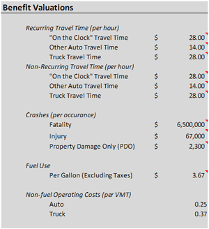
Source: FHWA TOPS-BC, 2012.

Estimating the Life-Cycle Costs

Estimating the costs of TSM&O strategies is often complex. Compared to more traditional infrastructure improvements, TSM&O improvements typically incur a greater proportion of their costs as continuing O&M costs, as opposed to upfront capital costs. Much of the equipment associated with TSM&O strategies also typically has a much shorter anticipated useful life than many traditional improvements, and must be replaced as it reaches obsolescence. Further complicating the TSM&O cost estimation process is the fact that TSM&O deployment costs are greatly impacted by the degree in which equipment and resources are shared across different deployments and jurisdictions.

Despite these difficulties, it is critical that planners fully consider and account for all the costs of TSM&O strategies when evaluating and developing deployment and O&M plans. Failure to recognize and accurately forecast these costs may result in future funding or resource shortfalls, or worse, the inability to properly operate and maintain deployed TSM&O improvements. The cost estimation capability developed within the TOPS-BC support tool is intended to assist planners in estimating and predicting high-level cost and resource requirements of planned TSM&O strategies.

A good structure to follow for organizing these cost data includes:

• Capital costs – Include the upfront costs necessary to procure and install equipment related to the Operations strategy. These costs will be shown as a total (one-time) expenditure, and will include the capital equipment costs, as well as the soft costs required for design and installation of the equipment.
• O&M costs – Include those continuing costs necessary to operate and maintain the deployed strategy, including labor costs. While these costs do contain provisions for upkeep and replacement of minor components of the system, they do not contain provisions for wholesale replacement of the equipment when it reaches the end of its useful life. These O&M costs will be presented as annual estimates.
• Replacement costs – Include the periodic cost of replacing/redeploying system equipment as it becomes obsolete and reaches the end of its expected useful life in order to insure the continued operation of the strategy.
• Annualized costs – Represent the average annual expenditure that would be expected in order to deploy, operate, and maintain the Operations strategy; and replace (or redeploy) any equipment as it reaches the end of its useful life. Within this cost figure, the capital cost of the equipment will be amortized over the anticipated life of each individual piece of equipment. This annualized figure is added with the reoccurring annual O&M cost to produce the annualized cost figure. This figure is particularly useful in estimating the long-term budgetary impacts of TSM&O deployments.

The complexity of many Operations deployments warrants that these cost figures be further segmented to ensure their usefulness. Within each of the capital, O&M, and annualized cost estimates, costs should be further disaggregated to show the infrastructure and incremental costs. These are defined as follows:

• Infrastructure costs – Include the basic “backbone” infrastructure equipment (including labor) necessary to enable the system. For example, in order to deploy a camera (closed-circuit television (CCTV)) surveillance system, certain infrastructure equipment must first be deployed at the traffic management center to support the roadside ITS elements. This may include costs, such as computer hardware/software, video monitors, and the labor to operate the system. Once this equipment is in place, however, multiple roadside elements may be integrated and linked to this backbone infrastructure without experiencing significant incremental costs (e.g., the equipment does not need to be redeployed every time a new camera is added to the system). These infrastructure costs typically include equipment and resources installed at the traffic management center, but may include some shared roadside elements as well.
• Incremental Costs – Include the costs necessary to add one additional roadside element to the deployment. For example, the incremental costs for the camera surveillance example include the costs of purchasing and installing one additional camera. Other deployments may include incremental costs for multiple units. For instance, an emergency vehicle signal priority system would include incremental unit costs for each additional intersection and for each additional emergency vehicle that would be equipped as part of the deployment.
  Structuring the cost data in this framework provides the ability to readily scale the cost estimates to the size of potential deployments. Figure 5-10 provides a sample view of the cost data organized according to the defined structure in the TOPS-BC application. Infrastructure costs would be incurred for any new technology deployment. Incremental costs would be multiplied with the appropriate unit (e.g., number of intersections equipped, number of ramps equipped, number of variable message sign locations, etc.); and added to the infrastructure costs to determine the total estimated cost of the deployment. Presenting the costs in this scalable format provides the opportunity to easily estimate the costs of expanding or contracting the size of the deployment, and allows the cost data to be reutilized for evaluating other corridors.

Figure 5-10. Example View of Cost Data Organization for a Ramp Meter System

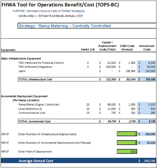
In the ramp meter example shown in Figure 5-10, the Annualized Costs for any individual piece of equipment equals the Capital Costs (which represents the total cost to deploy or redeploy that piece of equipment) and divided by the Useful Life (to amortize the cost of the equipment over the anticipated life), plus the annual cost of operating and maintaining the piece of equipment. This methodology assumes that the piece of equipment is redeployed at the end of its useful life. For example, the Annualized Costs for the equipment called “TMC Hardware for Freeway Control” is calculated as:

Annualized Costs = (Capital Costs/Useful Life) + Annual O&M Costs
or
Annualized Costs = ($22,500/5 years) + $2,000 = $6,500

Some equipment does not have upfront Capital Costs, but only has recurring annual O&M Costs, as illustrated by the “Labor” costs in the Figure 5-10 example. In these situations, the annualized cost is simply the annual O&M Costs.

In the TOPS-BC application, users are able to enter the quantity of Infrastructure and Incremental equipment units they want to deploy, as shown in Figure 5-10; and the tool will calculate the total cost of the selected deployments based on these entries. (For most TSM&O strategies, the number of “Infrastructure” deployments will be one, as only one deployment of this equipment is necessary to support multiple deployments of the “Incremental” units. However, the user has the opportunity to deploy more than one “Infrastructure” unit if their planned deployment is configured in a nontypical manner (e.g., managed from multiple Traffic Management Centers).) Average Annual Costs for the ramp metering example would be calculated as:

Average Annual Costs = (# of Infrastructure Deployments * Annualized Costs of Infrastructure Deployment) + (# of Incremental Deployments * Annualized Costs of Incremental Deployment)
or
Average Annual Costs = (1 * $296,500) + (10 * $5,990) = $356,400

Outputs from this process include the following:

• An Average Annual Cost – A single expected cost compiling upfront capital, ongoing O&M, and future equipment replacement costs in a single figure.
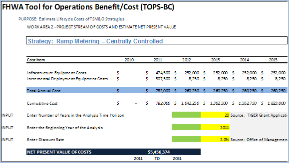
• A Projected Stream of Costs – An output showing year-by-year expected expenditures over the next 30-year timeframe. This stream of outputs will also have the capability to escalate future expenditures based on an inflation rate selected by the user. This output can be used to calculate Net Present Value (NPV) over any time horizon chosen by the user, if they chose to use NPV instead of average annual costs in their analysis.

Figure 5-11 shows a sample view of the Projected Stream of Costs generated for the ramp meter strategy illustrated in the earlier Figure 5-10. In this view, the Capital Costs are not amortized over the life of equipment, but appear in the year they are incurred. Upfront Capital Costs appear in the first year of deployment (as indicated by the user), and Replacement Costs are incurred in future years, as equipment needs to be replaced. In the case of the ramp metering example, the full Capital Cost of deployment is incurred in year 2010, but only a portion of the Capital Cost are incurred again in year 2015, since only a portion of the equipment involved in the deployment has reached the end of its useful life by this date. Space is provided to view costs up to a 50-year time horizon. The user may calculate the NPV of the costs by selecting a time horizon (in number of years) and an appropriate discount rate. Defaults are provided, but the user may override those defaults by entering their own values.

Figure 5-11. TOPS-BC Projected Stream of Costs Output

Displaying and Communicating Results

Although the primary output of a benefit/cost analysis is a relatively simple ratio (B/C ratio) and estimate of Net Benefits, there are typically many additional data regarding changes to various MOEs and costs that roll up into the B/C ratio that provide robust opportunities to present and explain the findings in order to promote better understanding and acceptance of the results. Prior to developing the presentation of findings, the analysts and project managers should carefully consider the following:

• What is (are) the key audience(s) for the results? If the primary audience is a technical one, the analysts should be prepared to present sufficient detail to allow the reviewers to map their own conclusions to the ones presented by the performing entity. If the audience is anticipated to comprise public or high-level decision-makers, the analyst may want to carefully craft a presentation of data to make effective use of graphics to display a high level of information in an easily digestible and understandable format. In many cases, the findings may need to be presented to differing audiences; and in these cases, different formats and data displays may be required.
• What is the key information to present? B/C analysis often results in significant amounts of data being generated regarding individual impacts to different MOEs. Attempting to present all this information can quickly result in overwhelming the audience and losing focus on the key issues. The analyst should attempt to identify the key issue or issues, appropriate to the intended audience, and focus the output display on those issues.
• How can graphics and charts be best used to condense multiple data? Charts and graphics can go far beyond simple pie charts and line graphs to effectively present information representing multiple data simultaneously in an easy to comprehend format – often times increasing the readers understanding of the relationship between multiple variables.

Figure 5-12 shows the innovative use of a graphic to simultaneously present multiple pieces of data comparing different projects. This graphic concurrently compares:

• The relative benefit/cost ratio estimated for the project (down the left axis);
• The relative size of the net benefit (by the size of the bubble);
• The number of qualitative goals met (across the bottom axis);
• The type of the project (by color); and
• The project name.

Figure 5-12. Innovative Use of Graphics to Display Multiple Data

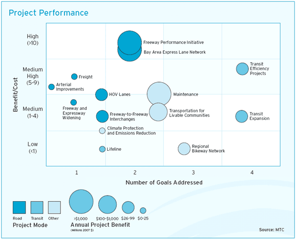
Source: San Francisco Bay Area MTC 2030 Project Performance Assessment, 2007.

Graphics can also be effectively used to present data occurring over a timeline for those analyses using a defined time horizon. Figure 5-13 presents estimated costs, separated by upfront capital costs and ongoing O&M costs shown against the left axis, over an 11-year time horizon. This graphic effectively portrays the concept that, as more capital costs are expended to deploy more operations strategies, the annual O&M costs continue and increase as a result of more and expanded strategies to manage. The right-hand axis of the graphic displays the cumulative capital costs over the project time horizon.

Figure 5-13. Sample Graphic Presenting Results over an Analysis Timeline

Source: Wisconsin DOT Traffic Operations Infrastructure Plan, 2007.

Addressing Challenges of Applying B/C Analysis to TSM&O Strategies Targeted at Nonrecurring Conditions

The concepts of travel time reliability and addressing nonrecurring congestion have increasingly been receiving attention in recent years. This is particularly important in regards to many TSM&O strategies since many are targeted specifically at nonrecurring conditions (e.g., incidents, special events, work zones, and inclement weather). Many of the traditional tools designed to analyze transportation projects, however, have proved to be ill-suited to analyzing nonrecurring conditions. For example, traditional travel demand models, which have historically shouldered a large portion of alternative analysis needs for many agencies, are typically developed and calibrated to days with good weather, no incidents, normal demand, and no work zone activity. This means that these traditional analysis methods do not consider the additional negative impacts (reduced capacity, speeds, increased crashes) related to these nonrecurring conditions; and as such, TSM&O strategies analyzed using these traditional methods may have their potential benefits severely understated.

As a result of the increasing focus on the significant portion of congestion caused by nonrecurring sources, and the ability of TSM&O strategies to effectively improve travel conditions during nonrecurring events, much improvement has recently been made in enhancing the analysis of nonrecurring conditions. Two national initiatives, in particular, have made significant advances in overcoming some of the analysis challenges related to identifying and quantifying nonrecurring congestion and the impacts of TSM&O strategies in mitigating the negative impacts. These initiatives include the FHWA ICM initiative, which includes the development of an Analysis, Modeling, and Simulation (AMS) Guide to aid practitioners at applying the developed analysis methods, and the ongoing FHWA development of a Guidebook on Analysis of Active Transportation and Demand Management Using Highway Capacity Methods.

These projects both are developing analysis methods related to multiresolution/multiscenario methods, which as discussed in Chapter 4, and represent the most complex methods best capable of assessing these types of impacts. Although much more complex in their actual application, these analyses follow several general steps, including:

1. The identification of the causes of nonrecurring congestion in a region;
2. The identification of the negative impacts of these nonrecurring conditions (e.g., reduced capacity caused by rainy conditions);
3. The modification of analysis models and routines to be able to model baseline nonrecurring scenarios;
4. The identification of TSM&O and traditional projects impact on these nonrecurring conditions;
5. The identification and incorporation of appropriate MOEs into the analysis that are capable of quantifying the benefits;
6. The adjustment and development of modeling tools and methods to support the analysis; and
7. The effective presentation and explanation of results.

Although more complex than many typical analysis that only consider recurring congestion, these enhanced analyses may be used to support B/C analysis of TSM&O strategies. The basic premise behind this method is to separately analyze recurring and various nonrecurring conditions as different scenarios, and then sum the results of all the scenarios, weighted to the frequency in which each individual scenario is anticipated to occur in a typical year. To accomplish this, the analyst will need to compile data on historic patterns for:

• Demand variability;
• Weather patterns;
• Incident occurrence; and
• Work zones.

In order to develop scenarios representing these nonrecurring conditions, the analyst will need to make modifications to the baseline parameters in the model used to reflect the capacity loss of these nonrecurring conditions. As part of the development of the Guidebook on Evaluation of Active Transportation and Demand Management Using Highway Capacity Methods, a number of baseline capacity constraints has been mapped to various nonrecurring conditions based on data in the 2010 HCM. Table 5-5 presents the capacity reduction factors related to various inclement weather conditions. Table 5-6 presents capacity reduction factors related to various incident types. Table 5-7 presents capacity reduction factors related to various.

Table 5-5 Capacity Reduction Based on Nonrecurring Weather Types

Weather Type	Capacity Range (Percentage)
Rain	2-14
Snow	4-22
Low temp	1-9
High wind	1-2
Visibility	1-12

Source: FHWA Guidebook on Analysis of Active Transportation and Demand Management Using Highway Capacity Methods – Workshop Presentation, adapted from Exhibit 10-15, 2010 HCM.

Table 5-6 Capacity Reduction Based on Nonrecurring Incidents (In Percentage)

Number of Lanes (1 Dir)	Shoulder Disablement	Shoulder Accident	One Lane Blocked	Two Lanes Blocked	Three Lanes Blocked
2	5	19	65	100	N/A
3	1	17	51	83	100
4	1	15	42	75	87
5	1	13	35	60	80
6	1	11	29	50	74
7	1	9	25	43	64
8	1	7	22	37	59

Source: FHWA Guidebook on Analysis of Active Transportation and Demand Management Using Highway Capacity Methods – Workshop Presentation, adapted from Exhibit 10-17, 2010 HCM.

Table 5-7 Capacity Reduction Related to Work Zones (In Percentage)

Original Lanes	Work Lanes
	1	2	3	4
1	?	N/A	N/A	N/A
2	67	?	N/A	N/A
3	77	54	?	N/A
4	84	65	46	?

Source: FHWA Guidebook on Analysis of Active Transportation and Demand Management Using Highway Capacity Methods – Workshop Presentation, adapted from Exhibit 10-14, 2010 HCM.

The capacity reduction factors, presented in the tables above, may be used to create various baseline scenarios that represent one or a combination of these various nonrecurring conditions. The development and analysis of additional scenarios representing different nonrecurring conditions needs to be carefully considered, however, as each additional scenario will require additional time and resources to create and run. In addition, it is important for the analyst to remember that, in order to conduct a B/C analysis of TSM&O strategies, each of the scenarios will need to be run twice, once as baseline without the strategy and once as an alternative scenario with the strategy deployed. Therefore, adding additional nonrecurring conditions scenarios can quickly multiply the number of model runs that are required.

It is recommended that the analyst review the data compiled on the frequency of nonrecurring events in order to develop a reasonable number of scenarios that may be modeled. Table 5-8 presents a sample comparison of the frequency of occurrence of various incident and bad weather conditions compared with varying levels of travel demand (presented as percentiles of the volume distribution), prepared for a sample section of the I-580 corridor in California as part of the development of the FHWA Guidebook on Evaluation of Active Transportation and Demand Management Using Highway Capacity Methods. These probabilities may be used to first assess the usefulness of analyzing particular scenarios – the used may decide to omit analyzing scenarios with very low likelihood of occurrence. Secondly, these probabilities may be used to weight the outcomes of individual scenarios – the analyst would apply a higher weight on those scenarios with a greater likelihood of occurrence.

Table 5-8 Sample Scenario Probabilities – I-580 Corridor

Capacity Reduction		5% Demand	20% Demand	50% Demand	80% Demand	95% Demand	Row Totals
No incidents, Good Weather	0%	6.04%	15.10%	18.12%	15.10%	6.04%	60.40%
Single Lane Closure, Good Weather	42%	2.16%	5.40%	6.48%	5.40%	2.16%	21.60%
Dual+ Lane Closure, Good Weather	75%	0.07%	0.19%	0.22%	0.19%	0.07%	0.74%
No incidents, Bad Weather	7%	1.26%	3.15%	3.78%	3.15%	1.26%	12.60%
Single Lane Closure, Bad Weather	49%	0.45%	1.13%	1.35%	1.13%	0.45%	4.50%
Dual+ Lane Closure, Bad Weather	82%	0.02%	0.04%	0.05%	0.04%	0.02%	0.16%
Column Totals		10.00%	25.00%	30.00%	25.00%	10.00%	100.00%

Source: FHWA Guidebook on Analysis of Active Transportation and Demand Management Using Highway Capacity Methods – Workshop Presentation, 2011.

The probabilities of various scenarios would be expected to vary depending on the region and even the individual corridor; therefore, it is recommended that analysts assemble and analyze the probabilities of nonrecurring conditions individually for each study. Once this data has been analyzed, the analyst can prioritize various scenarios to be developed and analyzed based on their probabilities. For example, if resources are not available to run all scenarios, the analyst may want to discard those strategies with very low probabilities.

Once all the scenarios have been analyzed for both the baseline and alternative scenarios, the incremental change in benefits for each scenario would be weighted according to its probability and summed to provide an estimate of benefits across all recurring and nonrecurring conditions.

Additional Resources and Support

The TRB Transportation Economics Committee recommends the following additional resources for supporting B/C analysis.

• Abley, S., P. Durdin, and M. Douglass, 2010, Integrated Transport Assessment Guidelines, Report 422, Land Transport New Zealand).
• American Association of State Highway and Transportation Officials (AASHTO), 2010, A Manual of User Benefit Analysis for Highways, Third Edition.
• Boardman, A., et al., 2005, Cost-Benefit Analysis: Concepts and Practice, Third Edition, Prentice Hall/Pearson.
• Caltrans, 2006, Benefit-Cost Models, Office of Transportation Economics, California Department of Transportation.
• Caltrans, 2007, Life-Cycle Benefit-Cost Analysis – Economic Valuations, California Department of Transportation, Division of Transportation Planning, Office of Transportation Economics.
• CASA, 2010, Cost Benefit Analysis Procedures Manual, Australian Government, Civil Aviation Safety Authority.
• Center for Transportation and the Environment (CTE), 2008, Improved Methods For Assessing Social, Cultural, and Economic Effects of Transportation Projects, NCHRP Project 08-36, Task 66, Transportation Research Board, AASHTO.
• DFID, 2003, Social Benefits in Transport Planning, UK Department for International Development. Describes methodologies for more comprehensive transportation project evaluation.
• DfT, 2006, Transport Analysis Guidance, Integrated Transport Economics and Appraisal, UK Department for Transport.
• EC, 2002, Guide to Cost-Benefit Analysis of Investment Projects, Evaluation Unit, DG Regional Policy, European Commission.
• EDRG, 2007, Monetary Valuation of Hard-to-Quantify Transportation Impacts: Valuing Environmental, Health/Safety and Economic Development Impacts, NCHRP 8-36-61, National Cooperative Highway Research Program.
• FAA, 1999, Airport Benefit-Cost Analysis Guidance, Federal Aviation Administration. U.S. Department of Transportation, Washington, D.C.
• FHWA, 2003, Economic Analysis Primer, Office of Asset Management, Federal Highway Administration.
• FHWA, 2001, Cost-Benefit Forecasting Toolbox for Highways, Federal Highway Administration, U.S. Department of Transportation, Washington, D.C.
• FMT, 2005, Federal Transport Infrastructure Plan 2003: Basic Features of the Macroeconomic Evaluation Methodology, German Federal Ministry of Transport.
• Forkenbrock, D. J., and G. E. Weisbrod, 2001, Guidebook for Assessing the Social and Economic Effects of Transportation Projects, NCHRP Report 456, TRB.
• Goodbody Economic Consultants, 2004, Cost Benefit Parameters and Application Rules for Transport Project Appraisal.
• GTKP, 2011, Economic Analysis for Multilateral Development Banks, Global Transport Knowledge Partnership.
• Hyder Consulting, 2008, Understanding Transport Costs and Charges (UTCC) Phase 1, New Zealand Ministry of Transport.
• Litman, T., 2001, What’s It Worth? Life Cycle and Benefit/Cost Analysis for Evaluating Economic Value, presented at Internet Symposium on Benefit-Cost Analysis, Transportation Association of Canada.
• Litman, T., 2010, Transportation Cost and Benefit Analysis, Victoria Transport Policy Institute.
• LTNZ, 2010, Economic Evaluation Manual (EEM), Land Transport New Zealand.
• Maibach, M., et al., 2008, Handbook on Estimation of External Cost in the Transport Sector, CE Delft.
• MSU, undated, Benefit/Cost Analysis: Introduction, Mankato State University.
• MNDOT, undated, Benefit Cost Analysis, MN DOT Office of Investment Management.
• Portney, P., undated, Benefit-Cost Analysis, The Library Of Economics and Liberty.
• TC, 2003-2007, The Full Cost Investigation of Transportation in Canada (multiple documents), Transport Canada.
• TRISP, 2005), Economic Evaluation Notes, UK Department for International Development and the World Bank.
• UNIDO, no date, A Guide to Practical Project Appraisal – Social Benefit-Cost Analysis in Developing Countries, United Nations.
• United Kingdom Department for Transport, Transport Analysis Guidance (WebTAG).
• van Essen, et al., 2004, Marginal Costs of Infrastructure Use – Towards a Simplified Approach, CE Delft.
• White House, 2003, Circular No. A-94: Guidelines and Discount Rates for Benefit-Cost Analysis of Federal Programs, Office of Management and Budget, U.S. Government, Printing Office, Washington, D.C.
• World Bank, 2008, A Framework For Urban Transport Projects: Operational Guidance for World Bank Staff, Transport Sector Board, World Bank.
• Zhang, A., A. E. Boardman, D. Gillen, and W. G. Waters II, 2005, Towards Estimating the Social and Environmental Costs of Transportation in Canada, Centre for Transportation Studies, UBC, for Transport Canada

You will need the Adobe Reader to view the PDFs on this page.