Traffic Analysis Toolbox Volume XII:
| ||||||||||||||||||||||||||||||||||||||||||||||||||||||||||||||||||||||||||||||||||||||||||||||||||||||||||||||||||||||||||||||||||||||||||||||||||||||||||||||||||||||||
| Intersection | Control Delay (Seconds) | LOS |
|---|---|---|
| MD 144 at Dutton Avenue | 144.9 | F |
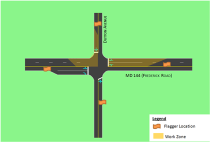
The alternate work zone model, developed by the agency, features a three-way flagging work zone layout. For this alternative, the eastbound and westbound approaches were changed to each have one shared left-through-right lane. These lanes would be shifted throughout the construction to permit the approaches to operate concurrently. This alternative’s work zone configuration is shown in Figure 41. To represent the three-way flagging operations, this alternative was modeled by changing the existing condition’s intersection control into an actuated-uncoordinated signal control with split phasing for the minor approaches. The model results for this alternative are shown in Table 84.
Figure 41. Three-Way Flagging Work Zone Configuration
(Source: Maryland State Highway Administration, 2008.)
| Intersection | Control Delay (Seconds) | LOS |
|---|---|---|
| MD 144 at Dutton Avenue | 22.2 | C |
As the results show in Table 84 Alternative 2 meets the mobility thresholds and is chosen as the recommended alternative. Additional analysis was performed in order to determine when it was best to implement the flagging operations. Table 85 presents the recommended work zone alternative and work hour restrictions.
Alternative Analysis Options
The alternative analysis process may differ based on the agency and the project. In this case, a second work zone alternative was considered because the primary alternative did not meet the mobility thresholds. Another alternatives analysis approach may involve analyzing several alternatives concurrently and then using a set of different performance measures to compare and choose among the alternatives. In this situation, the criteria for selecting the preferred alternative depended only on mobility thresholds. For other decision-making framework options, refer to Chapter 5 of this document.
This case study is based on the hypothetical application of Maryland SHA’s lane closure analysis methodology on I-95, an eight-lane, two-way divided interstate highway that runs in the north-south direction through Howard County, Maryland. This case study, featured in Maryland SHA’s Work Zone Analysis Guide, evaluates the impacts of a resurfacing project on both directions of I-95 approximately between MD 216 and I-895, as shown on Figure 42. (Work Zone Analysis Guide. Maryland State Highway Administration (SHA), Maryland, September 2008. Accessed January 11, 2012.) The roadway resurfacing excludes the ramps. The work is to be completed by resurfacing two travel lanes at a time and in one-mile-long segments.
Figure 42. I-95 Howard County, Maryland Study Area Map
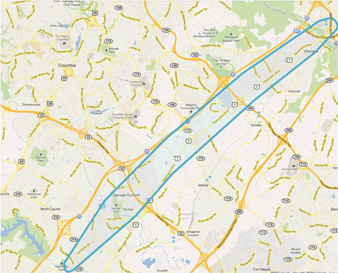
(Source: Maryland State Highway Administration, 2012.)
The objective of the analysis is to determine the time periods when it would be most appropriate for three lanes on the mainline to be closed.
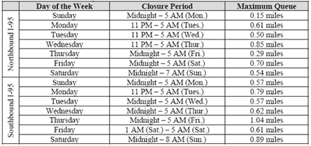
Performance measures and outputs extracted from the analysis include maximum queue length across different days of the week and lane closure durations. The freeway lane closure mobility thresholds established by the agency are that queue length should be less than one mile for any duration and that queues between 1 and 1.5 miles should last less than two hours.
Because of the simplicity of the work zone, the agency decided to perform the analysis using the lane closure analysis program (LCAP).
Analysis Tool Selection Options
In this case study, LCAP was chosen as the analysis methodology based on the level of complexity of the project. However, there are also additional factors that can be considered when selecting the analysis tool. Chapter 3 of this document describes these various factors in greater detail. The recommended factors for identifying the appropriate modeling approach include:
The analysis will determine which combinations of days of the week and lane closure durations will meet the threshold indicating when a three-lane closure is acceptable. There is an alternative for each day of the week per direction of traffic along I-95. Therefore, there are a total of 14 alternatives. Each of these alternatives is presented in Step 6.
During this stage of the modeling development and analysis, the analysts should define the objectives of the analysis, the scope of the modeling or analysis effort, and identify the data needed for the modeling analysis effort.
The next step of the MOTAA is to develop the existing conditions model. Because simulation modeling was not needed to analyze the study area, there was no need for an existing conditions model and calibration effort.
Due to the nature of this analysis, there was no need for model development for both the existing conditions as well as work zone base. Therefore, a calibration effort also was deemed unnecessary. For information on the analysis conducted, refer to Step 6, Alternatives Analysis.
Typically, if modeling was involved, the alternatives analysis step included two stages: 1) development of models to capture the scenarios or alternatives; and 2) description of how these models were run, the outputs extracted, and analysis of the results. In this case study, the stages are varied slightly. The first stage of this case study is to 1) determine the inputs to the LCAP analysis, and then 2) produce model outputs after running LCAP.
For this case study, the first stage of the work zone base conditions model development was to determine the input to the LCAP. One of the main inputs to the program is work zone capacity. There are three capacity approximations methodologies featured in LCAP:
Therefore, the average of the work zone capacity from these three equations equals 1,260 vphpl, the work zone capacity used for this analysis.
After determining the work zone capacity, the next stage is the development of an LCAP model using data such as existing traffic volumes, number of lanes (existing and work zone conditions), and capacity (existing and work zone). The model was set up assuming at least four consecutive hours will be needed for mobilization, resurfacing, and demobilization.
After setting up the model with the required inputs (detailed in Step 6A), the next step in the LCAP procedure is to run the program. With this case study several iterations were run using different combinations of closure time periods and days of the week to determine which periods in the day could accommodate a three-lane closure that would meet the agency’s mobility thresholds. The trial and error process is depicted by Figure 43 and Figure 44. Figure 43 shows one trial where the closure along I-95 northbound lasted from 10:00 p.m. Wednesday through 5:00 a.m. Thursday. This scenario or trial produced queues that violated the agency’s mobility thresholds. The other trial shown on Figure 44 depicts a more feasible alternative. A maximum queue length was determined for each alternative or combination. Figure 45 summarizes the maximum queue length associated with the lane closure duration for each day of the week.
Based on the results shown on Figure 45, the queues for each closure period meet the mobility threshold specified in Step 2. Therefore, the results show that there is at least one four-hour period every night that can accommodate a three-lane closure along I-95 for the resurfacing project.
Figure 43. I-95 NB, Howard County, LCAP Output Trial 1 – Closure from 10:00 P.M. Wednesday to 5:00 A.M. Thursday
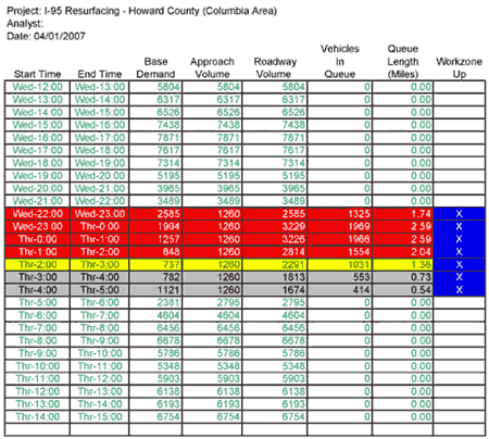
Figure 44. I-95 NB, Howard County, LCAP Output Trial 2 – Closure from 11:00 P.M. Wednesday to 5:00 A.M. Thursday
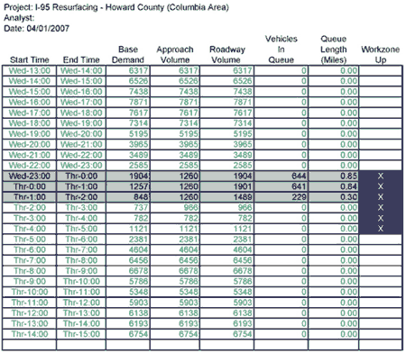
Figure 45. I-95 Howard County, LCAP Model Outputs
This case study describes the process used by Pesti, G., et al. (2010) from Texas Transportation Institute (TTI) to evaluate the impacts of two work zones on separate freeway corridors in El Paso, Texas, using a mesoscopic simulation tool. (Pesti, G., C. Chu, K. Balke, X. Zeng, J. Shelton, and N. Chaudhary. Regional Impact of Roadway Construction on Traffic and Border Crossing Operations in the El Paso Region. Texas Transportation Institute, October 2010.) Figure 46 shows the work zone locations of these two projects.
Figure 46. I-10/Loop 375 Case Study Project Area Map
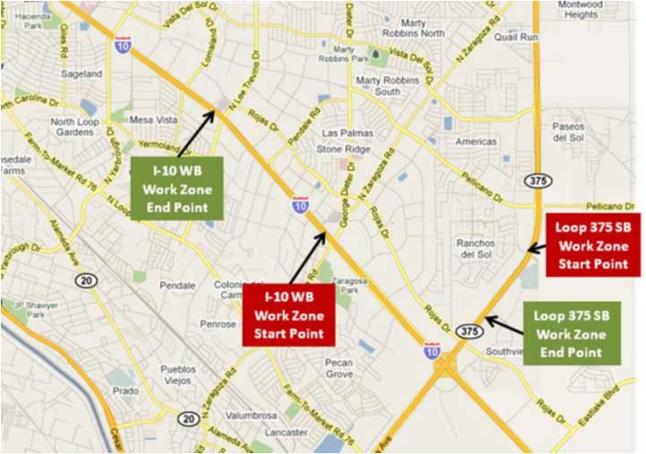
(Source: Pesti, Chu, Balke, Zeng, Shelton, and Chaudhary, 2010.)
The goal of the project was to determine the best construction sequence option that could minimize the disruption experienced by motorists.
The impact of construction was evaluated using LOS. The LOS criteria were based on HCM 2000. The criteria for freeways were based on densities and those for surface streets were based on link speeds.
Dynamic Urban Systems for Transportation (DynusT), a dynamic traffic assignment (DTA)-based tool, was used in the analysis. It was chosen because of its ability to evaluate the regional impacts of multiple work zone projects.
Analysis Tool Selection Options
In this case study, DynusT was chosen based upon the tool’s capabilities in evaluating the regional impacts of multiple work zone projects. Similar DTA-based tools can be applied for this case study as well.
Two project sequence options, with three scenarios, were evaluated in the case study; they are:
During this stage of the modeling development and analysis, the analysts should define the objectives of the analysis and identify the data needed for the modeling analysis effort. For this case study, the following types of construction data were collected:
The next step of the MOTAA is to develop the existing conditions model. The DynusT network was created in a separate Texas DOT Interagency Contract (IAC), in which the Texas Transportation Institute (TTI) converted the El Paso MPO’s “Trans-Border” travel demand model for the year 2009 into a format that can be used by DynusT. Note that this network was limited to the U.S. side of the border and did not include the City of Juarez, except a few external zones for the border crossing.
The DynusT network was represented by 2,862 nodes, 6,203 links, and 690 traffic analysis zones. The network was quite detailed and captured all freeways, interchanges, major arterials, and intersections that were included in the El Paso regional travel demand model. In addition, smaller localized minor roads were coded in the project study area. This additional level of detail was consistent with the scope of the project and scale of the problem that it tried to address.
Major elements of the DynusT network of the El Paso region were reviewed and checked to ensure that they correctly represented the existing roadway system of El Paso. Where needed, some network elements or origin-destination (O-D) matrix values were corrected and updated. After verifying the most critical elements of the network, several test runs were performed. The test runs were performed on the verified network and used a time-varying O-D matrix calibrated in a previous Texas DOT IAC project using an O-D calibration method developed by the University of Arizona.
The existing conditions model was then modified to represent work zone conditions. In this case study, there was no work zone base conditions model developed or calibrated.
Work Zone Base Conditions Model Development and Calibration
Work zone base conditions models may not be necessary. In this instance, the two work zone alternatives are compared against each other to determine the relative merits of each. As such, there is no need for a “base” to check against.
The alternatives analysis step involves two stages: 1) development of models to capture the scenarios or alternatives; and 2) description of how these models were run, the outputs extracted, and analysis of the results.
This case study featured three work zone alternative scenarios, which were created by modifying the existing conditions model.
The final steps of the MOTAA are to run the work zone alternative models using the selected traffic analysis tool and to extract select model outputs. As an example, Figure 47 shows lane-miles with LOS changes for Scenario 2.0, with C-C, N-C, and C-N representing traffic condition changes from congested to congested (C-C), noncongested to congested (N-C), and congested to noncongested (C-N).
Figure 47. I-10/Loop 375 Case Study – Lane-Miles with LOS Changes for Scenario 2.0
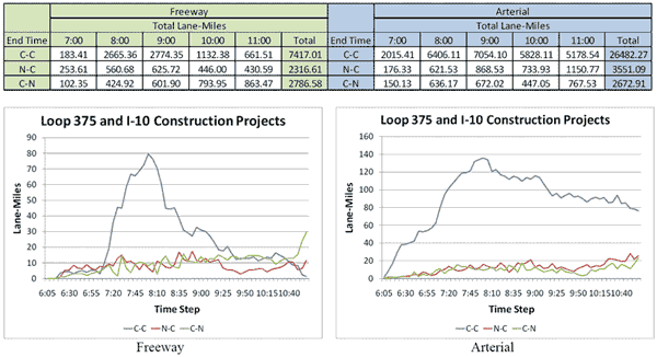
Note: Conduct both I-10 and Loop 375 projects simultaneously.
Based on the analysis, it was concluded that conducting the construction projects simultaneously had similar impact on traffic as the I-10 project alone. The I-10 project had greater negative impact than the Loop 375 construction. A significant portion of traffic would be diverted to the southern portion of the Loop 375 crossing I-10 during the I-10 construction phase. Lastly, the two projects had similar impacts to the arterial traffic.
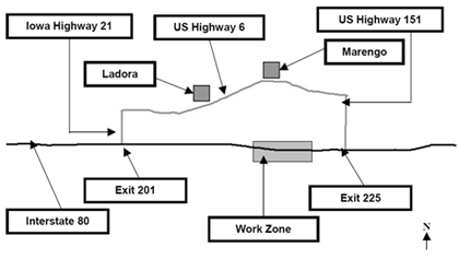
The following case study follows the research efforts and modeling analysis process employed by Schrock and Maze (2000) to evaluate the cost-effectiveness of delay-reducing work zone alternatives using microsimulation. (Schrock, D., and T. Maze. Evaluation of Rural Interstate Work Zone Traffic Management Plans in Iowa Using Simulation. Proceedings of the Mid-Continent Transportation Symposium, Iowa State University, Ames, 2000.) Schrock and Maze chose a completed Iowa DOT work zone project on rural Interstate 80 in Iowa County, Iowa, as a case study for this research effort and modeling analysis. This work zone project occurred in 1997 when a six-mile-long section of I-80 was selected for pavement rehabilitation. Between 1988 and 1997, traffic levels on I-80 had increased by 44 percent. With age and increasing traffic levels, several of the older sections along this corridor were in great need of rehabilitation and repair. The Iowa DOT, therefore, proceeded with the pavement rehabilitation efforts in 1997, converting the facility from a four-lane highway to a two-lane, two-way operation (TLTWO) between May 31, 1997 until September 13, 1997, when the project was completed. Figure 48 depicts the study area location and detour routes used.
Figure 48. I-80 Work Zone Study Area
The following sections describe how Schrock and Maze employed the MOTAA process into their research and modeling analysis of the I-80 pavement rehabilitation project in 1997. The process follows the MOTAA process, as described in Chapter 2 of this document, as well as the microsimulation modeling procedure described in Section 4.7.
The goal of this research and modeling effort was to evaluate different work zone alternatives through microsimulation in order to choose the most cost-effective strategy(s). Their objective was to compare the incremental benefits and costs of several hypothetical work zone alternatives against the actual 1997 I-80 pavement rehabilitation project to determine the alternative that would substantially reduce traffic congestion while efficiently using the resources allocated for the project. The researchers used the 1997 work zone data to develop a base case scenario that was then used to evaluate and compare the delays and costs associated with the various work zone alternatives.
After defining the goal and objective of the project, the next step in an MOTAA is to establish the MOEs and/or thresholds that would be used to evaluate and compare the different work zone alternatives. In order to compare and choose among these alternatives, the authors used MOEs, such as vehicle delay, travel time, user costs (costs due to delay), and agency costs. The researchers used these measures and converted them into dollar values for use in a benefit/cost analysis, which is described in further detail in Step 7.
The next stage of the MOTAA process is to determine the type of analysis tool to be used and justification for the selection. In this case study, microscopic simulation was used to determine the amount of delay that would occur under different alternative scenarios during the lifetime of the work zone. Traffic Software Integrated System (TSIS) CORSIM package was chosen because of its ability to provide the data outputs and measures required for the benefit/cost analysis. The authors felt that obtaining these outputs would have been difficult to obtain from other analysis tools.
Analysis Tool Selection Options
Although performance measures is one factor that should be considered in determining which tool is appropriate for a work zone traffic analysis, there also are other factors that should be considered before making the final decision. Chapter 3 of this document describes these various factors in greater detail. The recommended factors for identifying the appropriate modeling approach include:
After determining the MOEs and the analysis tool, the next stage of an MOTAA process is the identification of work zone alternatives. In this case study, the researchers developed several alternatives that were compared against the base case or “Do-Nothing Alternative.” The authors developed the following alternative scenarios:
At this stage of the MOTAA, the analyst already should have defined the objectives of the project and selected an appropriate tool that would be best for the project goals, objectives, and performance measures established. The next step of the MOTAA is defining the procedures necessary in preparing for modeling analysis. One of the first model preparation steps necessary is data collection. In this case study, the data collection efforts included:
Demands (Entry Volumes and O-D Tables) Options
This case study did not require the need for O-D tables. When using other microsimulation software, O-D estimation may be needed. Refer to Chapter 4 of this document for further details regarding the O-D estimation process.
The next stage of the microsimulation modeling process within an MOTAA procedure is typically the development of the existing conditions model, which often emulates the preconstruction condition in the project area. This is then usually followed by a model calibration effort. Because this case study conducts the MOTAA process after the project has been completed, the researchers do not build an existing conditions model. Instead they proceed to Step 5D, the work zone base conditions model development.
After the existing conditions model development and calibration effort, the following step in an MOTAA process is typically the development of the work zone base conditions model. If an existing conditions model already has been developed, the work zone conditions model usually involves the modification of the previous model using data regarding road and lane geometric configurations, signal controls, traffic demands, and capacity changes associated with the presence of the work zone.
In this case study, the work zone base model or the “Do-Nothing” alternative was developed using the FRESIM component of the TSIS software package. The network model covers the six-mile section of I-80 with one lane blocked in each direction by an incident as a way of simulating the work zone location. The highways that make up the detour network were created using the NETSIM portion of the TSIS software.
Error Checking in Model Development
Although not specified in this case study, during model development, the analyst should make sure to perform error checks to identify and correct any model coding errors. The analyst can check the model network geometries and traffic control operations against existing plans or engineering drawings.
After the development of the work zone base conditions model, the next stage in the modeling effort is typically a work zone base conditions model calibration. The work zone model calibration’s purpose is to ensure that the model is sufficiently able to reproduce the local driver behavior, traffic characteristics, and work zone capacity during the project’s duration. Because the modeling efforts conducted in this case study occurred after the work zone project was completed, the authors were able to calibrate their Do-Nothing model alternative using data collected during the implementation of the pavement rehabilitation project. The model was calibrated to the traffic conditions present when the work zone was active using the traffic data specified in the data collection section.
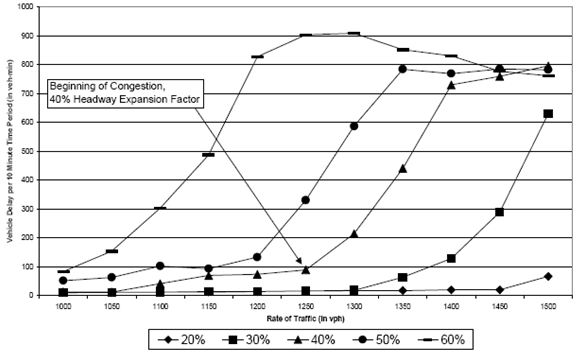
To appropriately model traffic behavior within the work zone area, adjustments and tests were conducted by varying the modeling tool’s headway factor parameter values. To determine the appropriate headway adjustment factor, the researchers used a one-directional, two-lane interstate test section to run a sensitivity analysis that assessed the impacts of various values of the headway factor. A hypothetical work zone was placed in the middle of the test section closing one lane of traffic. The work zone section had a speed limit of 55 mph and the rest at 65 mph. In this sensitivity analysis test, the headway factor was adjusted in increments of 10 percent between the values of 20 percent and 60 percent. The first iteration of the test started at a headway factor of 20 percent. Traffic volumes were input into the model using the traffic generator at a rate of 1,000 vehicles per hour (vph) with 20 percent trucks. The volumes were then increased by small increments up to a maximum of 1,500 vph at regular time intervals during the simulation. The test was repeated for the other headway adjustment factor increments of 30 percent, 40 percent, 50 percent, and 60 percent. The results were then analyzed to determine when delays began for each percentage of headway increase. Figure 49 depicts the results of the delay analysis for the various headway factor increments.
The results of the sensitivity analysis showed that a 40 percent increase in work zone headway can be associated with a vehicle delay beginning at about 1,250 vph, as shown in Figure 49. The capacity associated with the 40 percent headway factor parameter agrees with the results of a study conducted by the Iowa State University’s Center for Transportation Research and Education (CTRE) on the capacity of rural Iowa interstate work zone, which showed typical work zone capacities between 1,216 to 1,302 vph. The 40 percent headway factor was, therefore, deemed most appropriate for the calibrated work zone model.
Sensitivity Analysis Options
In this case study, the authors conducted a sensitivity analysis using varying headway expansion factors. Other driver behavior model parameters could also be used for sensitivity analyses and work zone base conditions model calibration processes. Chang and Zou (2009) conducted a sensitivity analysis using CORSIM testing three parameters: free flow speed, rubbernecking factors, and car-following sensitivity in order to calibrate a model to work zone conditions in the field. For further information on this research effort, refer to the Maryland State Highway Administration Research Report, Project SP708B4B, An Integrated Work-Zone Computer System for Capacity Estimation, Cost/Benefit Analysis, and Design of Control. (Chang, G.L., and N. Zou. An Integrated Work-Zone Computer System for Capacity Estimation, Cost/Benefit Analysis, and Design of Control. Maryland State Highway Administration, Project No. SP708B4B, Maryland, December 2009.)
Figure 49. Delay Associated with Varying Headway Expansion Factors
After the work zone model calibration, the analyst can proceed with modeling the alternatives analysis scenarios. The first step in this process is to create new models that reflect each alternative. This will require taking the “do-nothing” or base model and making the appropriate network model revisions. Afterwards the analyst will need to run the model alternatives multiple times, review the output, and extract relevant performance measures to be used in the next stage, the Decision-Making Framework.
CORSIM was used to develop and simulate the congested days condition for the six different alternatives (three alternatives and three sub-alternatives).
As previously mentioned, CORSIM software was used to perform the simulation runs for this stage of the analysis. Simulation runs were performed to model the 34 congested days for the six different alternatives. Additionally, five simulation runs were conducted for each day and alternative using different random seed numbers. The average total delay for each of the model alternatives was calculated, as shown on Table 86. The table presents the average delay, standard deviation, minimum value, maximum value, and range of delay for each alternative.
Number of Runs
In this case study, the authors decided upon five simulation runs. However, FHWA recommends an iterative approach that determines the appropriate number of model runs. For more information regarding this process, refer to Section 4.2 of this document or Traffic Analysis Toolbox Volume III. (A Primer for Dynamic Traffic Assignment. ADB30 Transportation Network Modeling Committee, Transportation Research Board, 2010.)
After obtaining the model output and mobility performance measures through the modeling analysis, the next stage of the MOTAA process is the application of a decision-making framework or criteria for evaluating and identifying the preferred alternative. In this case study, the researchers used the simulation results in a benefit/cost analysis (BCA). For further information on BCA and other decision-making frameworks that can be used during an alternatives analysis, refer to Chapter 5 of this document.
In order to convert the model delay values into dollar values, the authors used a previous Iowa DOT-sponsored study regarding the value of time. Table 87 shows the 1997 dollar values associated with delay. To determine the incremental benefits of each alternative to the Do-Nothing Alternative, the researchers determined the travel time savings that could be achieved for each scenario by determining the difference between the delay associated with the base scenario and the work zone alternatives. The delay differences were then converted to dollar values using the travel time value estimates shown in Table 87. The incremental cost represents the difference between the alternative’s project costs when compared to the Do-Nothing Scenario. The comparisons between the incremental benefits and costs for each alternative are shown in Table 88.
| Minutes | Average Value |
|---|---|
| 0 to 5 | $5.37 |
| 5 to 10 | $8.06 |
| 11 or more | $10.74 |
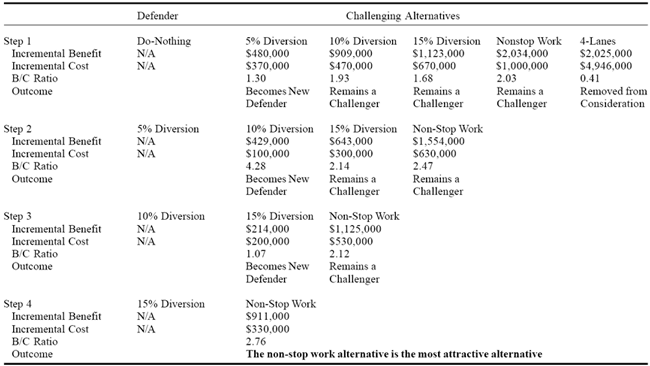
The BCA was completed in four stages as shown in Figure 50. In the first BCA step, the incremental benefits and costs of each alternative was compared to the Do-Nothing or Base Case Scenario. In the first step, the four-lane alternative was removed from consideration as the costs of the project far outweighed the benefits as seen by its BCA ratio of 0.41. The next option chosen in this step is the 5 percent Diversion alternative since it showed to have the lowest incremental cost as compared to the other alternatives. In the second iteration of the BCA, the incremental benefits and costs of each alternative are compared against the 5 percent Diversion alternative. The other alternatives still show a benefit over the 5 percent Diversion, with the 10 percent Diversion as the next option. The iteration is continued until the optimal case is found. In this exercise, the Nonstop Work alternative has an incremental BCA ratio of 2.03 when compared against the Do-Nothing alternative, and continued to be the most cost-effective throughout several iterations of the BCA comparison steps, as shown in Figure 50.
Figure 50. Summary of Benefits and Costs for each Alternatives
The following case study, along Interstate Highway 40 in North Carolina was featured in a research report completed by the Institute for Transportation Research and Education (ITRE) and sponsored by the North Carolina DOT Research and Development Group. (Schroeder, B., N. Rouphail, S. Sajjadi, and T. Fowler. Corridor-Based Forecasts of Work-Zone Impacts for Freeways. North Carolina Department of Transportation, Research and Analysis Group, Final Report Project 2010-08, 2011.) The purpose of the research effort was to develop an analysis methodology for the evaluation of significant work zone impacts on North Carolina freeways using FREEVAL-WZ. The report demonstrates the capabilities of FREEVAL-WZ, a deterministic software tool that implements the freeway facility methodology featured in HCM 2010.
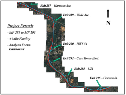
The report utilized the I-40 road widening project (STIP I-4744) in order to demonstrate the use of FREEVAL-WZ. For the purposes of this document, the I-40 example will be used as a case study to demonstrate the MOTAA process with urban freeway lane closure projects using FREEVAL-WZ for analysis. This work zone project involved an 18-month road widening by adding travel lanes in each direction of I-40 between State Road 1728 (Wade Avenue, Milepost 289) and the interchange with I-440/U.S. 1-64 (Milepost 293). The study area is shown by Figure 51. This segment of I-40 measures approximately 11.5 miles and includes a variety of different cross-sections (spanning two to four lanes per direction) of freeway segments, merge and diverge sections, and freeway weaving segments.
The research objective of the NC DOT report in conducting the work zone traffic analysis of the I-40 project was to demonstrate the use of FREEVAL-WZ and evaluate its capability to replicate field-observed work zone conditions. Therefore, the goals and objectives of this analysis differ from a case study project that would have or has been implemented in the field. An analyst may still use the methodology specified in this section in order to achieve certain project goals and objectives such as minimizing the mobility impacts on the freeway during construction.
Figure 51. I-40 Case Study Project Overview
The facility MOEs reported for this case study included average travel time, mainline travel speed, and capacity.
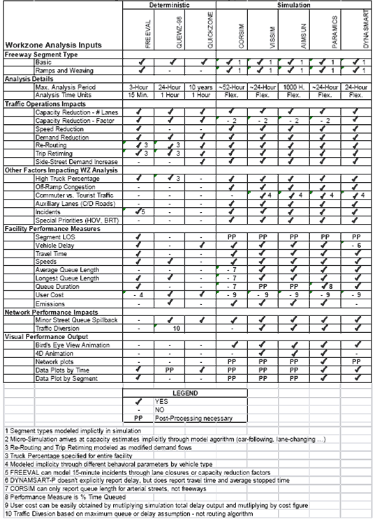
In the NC DOT report, the authors compared various analysis tools to FREEVAL-WZ. The authors first compared FREEVAL-WZ to other HCM/Deterministic tools. The authors note that while other deterministic tools such as QUEWZ-98 and QUICKZONE are limited to evaluating freeway segments, FREEVAL-WZ is able to evaluate demand changes on ramps and weaving segments in addition to freeways. Additionally, while the other tools have broader level, extended time periods for analysis, FREEVAL-WZ can be used as a peak hour analysis tool. Other differences between FREEVAL-WZ and other deterministic tools include output features and work zone-specific adjustments not available in other tools. These comparisons can be used by agencies and analysts to determine which deterministic tool is best suited for their project.
The authors also compared FREEVAL-WZ to simulation analysis tools such as mesoscopic and microscopic simulation software packages. While these tools can simulate and analyze the stochastic nature of traffic in relation to the work zone, there are certain advantages in using deterministic tools over simulation packages. For instance, the authors note that simulation tools can be more difficult to calibrate and are more data, time, and resource intensive as compared to deterministic tools. Therefore, depending on the analysis objectives, the level of complexity and detail needed for the analysis, and resource needs, an agency can determine which tool would be best suited for their project.
There also are new features and capabilities featured in FREEVAL-WZ that may add to an agency’s tool selection considerations. FREEVAL-WZ features a planning-level interface that allows agencies to customize the tool based on the agency’s needs and data resources. For instance, in the previous version of FREEVAL, traffic demand flows were required to be inputted into the tool as 15-minute increments. In the HCM 2010 version within the Planning-Level Analysis Module, traffic flows can now be directly inputted as average annual daily traffic (AADT), which is commonly used in planning-level analyses.
The authors also provided a summary table for comparing the capabilities of FREEVAL-WZ and other analysis tools in capturing work zone-specific impacts, shown in Figure 52.
Analysis Tool Selection Options
In this case study, FREEVAL was chosen based upon the tool’s capabilities in meeting the data and performance measures typically required in the agency’s work zone traffic analysis projects. Additionally, this option was also chosen based on the resource and data needs requirements of the tool as compared with other tool types. There are also additional factors that can be considered in selecting a tool. Chapter 3 of this document describes these various factors in greater detail. The recommended factors for identifying the appropriate modeling approach include:
Figure 52. Work Zone Impacts and Analysis Tools
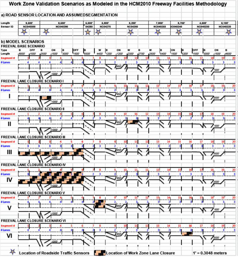
For the I-40 case study, several scenarios were developed, including an existing conditions scenario during the p.m. peak as well as nighttime and weekend lane closure scenarios. All of the lane closure scenarios (Scenarios 1 through 6) were evaluated from 9:00 p.m. to 12:00 a.m. Lane closures were scheduled to take effect at 9:00 p.m. but often did not start until 10:00 p.m. The lane configurations of the base and lane closure scenarios are featured in Figure 53. The six scenarios included the following:
For the modeling effort of the I-40 case study, the authors developed a FREEVAL-WZ model that would include only the eastbound direction of the facility. In order to develop these models, the authors first had to conduct a data collection effort to obtain road geometry, volume, and traffic controls and operations data.
Figure 53. HCM 2010 FREEVAL-WZ, I-40 Case Study Scenarios
(Source: Schroeder, Rouphail, Sajjadi, and Fowler,2011.)
Data Collection for Development of Models
The data collection effort for model development included inputs for the following:
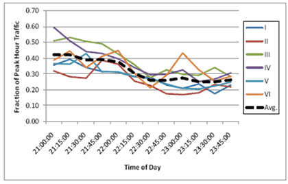
Figure 54. I-40 Work Zone Scenarios Demand Profiles
(Source: Schroeder, Rouphail, Sajjadi, and Fowler,2011.)
Data Collection for Validation and Development of FREEVAL-WZ Defaults
As previously mentioned, the main objective of the analysis was to evaluate how well FREEVAL-WZ could capture field-observed results. Therefore, in the initial stages of the project, significant traffic studies were performed in order to develop traffic stream models and capacity estimates for work zone operations specific to North Carolina. The initial studies involved an extensive data collection effort that analyzed sensor data regarding free-flow speeds, capacity, speed-flow relationships, segment speed and density, and travel time for various scenarios under freeway work zone conditions. During this stage of the modeling development and analysis, the authors utilized the following sources of information:
The field data provided traffic operations information such as speeds, capacity, and travel times for various work zone scenarios (these included different work zone lane closure configurations at various times of the day). They also aided the authors in developing plots that explained expected temporal distributions and speed-flow relationships by work zone scenario. Finally, analysis of the data also contributed to the development of capacity adjustment factors for each of the work zone scenarios. Such data were used to develop defaults for FREEVAL-WZ and were used to validate model results against field observations.
The next step of the MOTAA is to develop the existing conditions model with the appropriate geometry, traffic controls, demands, and capacities using the information from the data collection effort. To input the network geometry into FREEVAL, the analysts followed the methodology outlined in the HCM 2010 that divides a freeway facility into separate segments within four categories: Basic Segment, On-Ramp Segment, Off-Ramp Segment, and Weaving Segment. As shown in Figure 55, the facility is divided into 20 analysis segments. As mentioned in the previous step, traffic volume data for the p.m. peak hour was received from North Carolina DOT. As specified in Step 5A, additional processing was required in order to develop demand profiles for the off-peak lane closure scenarios.
The base model calibration/validation effort was performed using the operational analysis function of FREEVAL-WZ. Calibration of peak hour conditions was conducted by comparing field observed data (specified in Step 5A) to FREEVAL-WZ base model performance. One of the key measures used for calibrating the base model was travel time. The travel time target was the average facility travel time for the three-hour analysis period and the maximum 15-minute travel time across the facility. Field observed travel times were compared to the model’s travel time outputs.
In addition to travel times, the base model also was calibrated to speed data. Model speeds were calibrated using a visual comparison of space-mean speed plots or speed contour plots. Speed contour plots were generated for the existing conditions model and the work zone base conditions model. These were then compared to speed contour diagrams developed for four peak hour weekday work zone scenarios (generated using sensor data). The speed contour plots comparison is shown in Figure 55.
Model Calibration using Sketch-Planning and Deterministic Tools
Model calibration of sketch-planning and deterministic tools is typically conducted at a higher level and is often less time-consuming and resource-intensive as the calibration of macro-, meso-, and microscopic simulation models. The analysts’ calibration/validation procedure of comparing model outputs with field observations is typical for models developed with this tool type.
Figure 55. Speed Contour Plot Comparisons
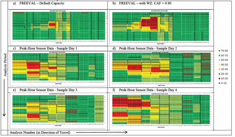
(Source: Schroeder, Rouphail, Sajjadi, and Fowler,2011.)
The PM Peak Work Zone Base, Barrier Work model follows the same configuration as the p.m. peak existing conditions model. The p.m. peak barrier scenario differs from the existing conditions model in that it represents construction activities along the corridor with reduced shoulder widths.
Calibration of the PM Peak Barrier Work model followed the same procedure as the existing conditions model. Calibration of the off-peak work zone scenarios were conducted using measures such as capacity, travel time, and speed contour plot comparisons.
Figure 56. I-40 Case Study Work Zone Scenarios Travel Time Comparisons
Figure 57. I-40 Case Study Work Zone Scenarios Capacity Comparisons
The alternatives analysis step involves two stages: 1) development of models to capture the scenarios or alternatives; and 2) description of how these models were run, the outputs extracted, and analysis of the results.
The work zone alternatives or model scenarios were developed as a result of the work zone diaries obtained from the contractors (work zone diaries are described in further detail in Step 5A). Using the work zone diaries and sensor data, the authors were able to determine the lane closure scenarios that occurred during construction. The six-lane closure scenarios detailed in Step 4 resulted from this analysis. The inputs and geometric configuration of these six scenarios are shown in Figure 58.
Figure 58. I-40 Case Study Work Zone Scenarios Speed Contour Comparisons
(Source: Schroeder, Rouphail, Sajjadi, and Fowler,2011.)
The final step of the MOTAA is to run the work zone alternative models and evaluate the performance measures extracted. The analysts used MOEs such as capacity, travel time, and comparisons of space-mean speed contour diagrams. Details regarding how these measures were extracted from the model are provided in Step 5D. As previously mentioned, the main objective of the analysis is to determine the capability of the FREEVAL-WZ models to capture and/or replicate field-observed work zone conditions and operations. As a result, the work zone scenarios were compared to field-observed conditions/data instead of to each other. Results of these comparisons are shown on Figure 56, Figure 57, and Figure 58.
Because the purpose of the ITRE report and the case study was to demonstrate the use of FREEVAL for work zone traffic analysis, the authors do not provide a recommended alternative. Therefore, no decision-framework was applied.
This case study features a benefit/cost (B/C) assessment of the temporary ITS used for the I-496 reconstruction project conducted for Michigan DOT. (Cambridge Systematics, Inc. Benefit/Cost Analysis of the Temporary Intelligent Transportation Systems (ITS) for the Reconstruction of I-496. Lansing, Michigan, November 2001.) The Michigan DOT undertook a major effort to repair and rebuild parts of the I-496 corridor through downtown Lansing. The reconstruction project, which began in April 2001 with a total value of the investment of $42.4 million, covered the I-496 corridor from the I-96 interchange on the west, to Trowbridge Road in the City of East Lansing. A map of the construction project is shown in Figure 59.
Figure 59. I-496 Case Study Project Area Map

Figure 60. I-496 Reconstruction Project Phasing

Both stages of this massive highway construction project resulted in major changes in commuting patterns. Therefore, Michigan DOT embarked on a concerted effort to help employers and residents of the Lansing region cope with this major reduction in capacity of the region’s transportation system. In addition to public education and outreach campaign, the following were the major efforts that were undertaken by Michigan DOT to mitigate the impacts of the construction project:
This study focused on a benefit/cost (B/C) assessment of the TTMS used for the I-496 reconstruction project. Michigan DOT intended to use the lessons learned through the TTMS deployment and its B/C evaluation to assist in decision-making for the procurement and deployment of such systems in the future.
The primary goals and objectives of this case study were outlined as follows:
The following performance measures were used to identify the impacts and benefits of the system:
The analysis used IDAS, a tool used to estimate the regional impacts and benefits of ITS deployments. IDAS was developed by FHWA and is intended to make the estimation of impacts and benefits of ITS deployments compatible with the methods used for other transportation projects. It utilizes existing regional travel demand models as the primary inputs for the analysis. The IDAS model is equipped with a comprehensive “ITS Benefits Database,” which consists of nationally and internationally reported benefits of ITS deployments over several years. The IDAS ITS benefits database is the primary source of impacts and benefits.
Analysis Tool Selection Options
In this case study, IDAS was chosen based upon the tool’s capabilities in estimating the impacts and benefits of ITS deployments, which was required by the agency (Michigan DOT). There also are additional factors that can be considered in selecting a tool. Chapter 3 of this document describes these various factors in greater detail. The recommended factors for identifying the appropriate modeling approach include:
This case study differs from a typical work zone analysis as it was specifically to conduct a benefit/cost assessment of the predetermined TTMS and arterial signal systems upgrades. Therefore, no other alternatives were analyzed.
During this stage of the modeling development and analysis, the analysts should define the objectives of the analysis and identify the data needed for the modeling analysis effort. For this case study, the following types of traffic data were collected:
The next step of the MOTAA is to develop the existing conditions model. The IDAS model was developed based on the travel demand networks and trip tables provided by the Tri-County Regional Planning Commission (TCRPC), which is the MPO for the three-county (Ingham, Eaton, and Clinton Counties) Lansing metropolitan region. The Lansing travel demand models were updated in 2000.
The IDAS model was validated by comparing the Vehicle-Miles Traveled (VMT) values generated by IDAS with those from the regional travel demand model.
Model Calibration using Sketch-Planning and Deterministic Tools
Model calibration of sketch-planning and deterministic tools is typically conducted at a higher level and is often less time-consuming and less resource-intensive than the calibration of macro-, meso-, and microscopic simulation models.
The travel demand models provided by TCRPC were then altered to reflect the freeway closure and lane closure of the two phases of the I-496 reconstruction project. A similar analysis performed by the Michigan DOT Central Office on an older version of the Lansing travel demand model was used as the template for representing the field conditions during the construction project. The disbenefits or negative impacts of the I-496 reconstruction project, obtained by running these networks in IDAS were documented.
There was no calibration data available for this work zone scenario. Therefore, there was no calibration efforts conducted that compared the work zone base with field conditions or with results from previous work zones of similar types.
The ITS components were deployed on each of the travel demand models, and IDAS was run to estimate the impacts and benefits of the deployment. The impacts of the deployments on the different travel performance measures were documented and the benefit/cost ratio was then calculated by comparing the benefits of the deployments with the total cost.
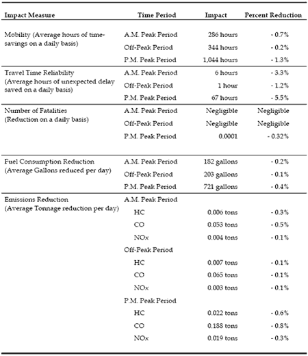
As described earlier, the benefits of the Temporary Traffic Management System (TTMS) include four categories: 1) user-mobility savings; 2) travel time reliability savings; 3) accident savings; and 4) emissions savings. For instance, the benefits for Phase 1 of the TTMS and the Arterial Signal System Upgrades are summarized in Figures 61 and 62, respectively.
Because the purpose of the study was to conduct a benefit/cost assessment of the predetermined TTMS and arterial signal systems upgrades for work zone traffic analysis, no alternatives were available and, therefore, it was not necessary to provide recommended alternative. Hence, there is no decision-framework applied.
Figure 61. I-496 Case Study – TTMS Benefits Summary (Phase 1)
Figure 62. I-496 Case Study – Arterial Upgrades Benefits Summary (Phase 1)
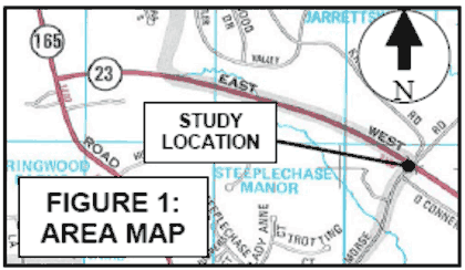
This case study, featured in the MD SHA Work Zone Analysis Guide (2008), describes the agency’s recommended MOTAA procedures for analyzing a two-way, one-lane bridge operation work zone project. (Work Zone Analysis Guide. Maryland State Highway Administration (SHA), Maryland, September 2008. Accessed January 11, 2012.) The hypothetical project is located on MD 23, a two-lane, two-way roadway that runs in the east-west direction over Morse Road. As with the flagging operations case study featured in Section 9.1, the main purpose of this and other case studies featured in the MD SHA Work Zone Analysis Guide is to demonstrate the application of the recommended MOTAA approach and guidelines.
Figure 63 depicts the study area location and nearby facilities. The nearest intersection to this bridge is where MD 23 terminates at MD 165, as shown in the project area map. There are no other access points between MD 23 and MD 165 west of Morse Road. The proposed work is to reconstruct the full length (100 feet) of the bridge.
As previously mentioned, this case study features the reconstruction of the MD 23 bridge over Morse Road. Because of the lack of access, there are no detour routes available, posing a challenge to mitigating the mobility impacts of the construction work. It is, therefore, assumed that the construction work would need to be accomplished through a two-stage process, where one lane at a time would be closed on the bridge, permitting traffic to flow on the other lane.
For this bridge reconstruction case study, the objective of the analysis is to determine if the reconstruction of the bridge performed using the one-lane, two-way bridge operations with traffic signals on either end could meet the mobility thresholds. Although this process notes that traffic signals would be used to regulate the flow of traffic on the one open lane, the analysis procedure featured in this section also could be applied for flagging operations.
Figure 63. MD 23 Case Study Project Area Map
In this case study, the mobility threshold is set at a 15-minute travel time increase limit. The measures of effectiveness included control delay and travel time.
Most arterials and freeways across the State of Maryland have been modeled using Synchro and CORSIM, respectively. To reduce data collection and model development efforts, Synchro was, therefore, chosen as the analysis tool.
Analysis Tool Selection Options
For this case study, Synchro was chosen because it reduced agency resource requirements and data collection efforts. Chapter 3 of this document describes other factors that can be considered when determining what type of analysis tool to use for the MOTAA. The recommended factors for identifying the appropriate modeling approach include:
In this case study, the agency did not predetermine a set of alternatives earlier on in the project. The first work zone scenario evaluated is the one-lane, two-way bridge operations with traffic signals on either end. A second work zone alternative is established should the primary scenario not meet the threshold. In this case study, no second work zone scenario was established because the primary scenario met the mobility thresholds, as shown in Step 6.
The goals and objectives of the analysis were described in Step 1 of this section. After determining the goals and objectives of the analysis, the next step includes determining the scope of the analysis (identifying the geographic boundaries of the study area) and the data inputs required.
Because there were no existing intersections at or near the study area, no model was created for existing conditions.
No existing conditions model was built. Therefore, there was no need for an existing conditions calibration process.
Model Calibration and Validation Options
If an existing conditions model calibration process is needed, each traffic signal optimization software package has a set of user-adjustable parameters that enable the analyst to calibrate the software to better match specific local conditions. The calibration process involves the selection of a few parameters for calibration and the repeated operation of the model to identify the best values for those parameters. Additionally, each agency and project may have different calibration guidelines and requirements. Section 4.4 of this document provides guidance on the considerations and steps involved in the calibration of traffic signal optimization models.
The next step in the MOTAA is the development of a work zone base conditions model. The one-lane bridge operations layout is shown in Figure 64. Model development for this case study includes considerations for geometric and signal controls.
![]()
Where:
C = Total cycle length;
G = Cumulative green time per cycle for both directions;
V = Total hourly volume for both directions; and
CL = Total clearance interval for each direction.
Figure 64. MD 23 Case Study – One-Lane Bridge Operations Layout
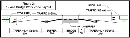
(Source: Maryland State Highway Administration, 2008.)
No work zone base conditions model calibration was conducted for this case study.
Work Zone Base Conditions Model Calibration Options
Work zone model calibration includes the calibration of work zone capacity and performance measures. Work zone model capacity and performance measures can be calibrated to field data and/or prior experiences (from similarly implemented work zone projects). In order to calibrate to field data or case studies of similar work zone types, the analyst will evaluate the work zone’s queues, travel times, delays, and speeds. Additionally, the analyst may study parameters related to driving behaviors in work zones of similar types. Such observations and measures will aid the analyst in the work zone calibration process.
The next step is to perform model runs in order to analyze the different alternatives. The analysis involves running the model and obtaining outputs and measures such as control delay. The control delay results for the one-lane bridge operations during both peak periods are shown on Table 90.
| Approach | Control Delay (Seconds) | |
|---|---|---|
| AM Peak | PM Peak | |
| Eastbound | 195.2 | 221.4 |
| Westbound | 188.3 | 196.2 |
The next step applied for this case study was to determine if the alternative meets the agency’s established mobility thresholds. According to the mobility thresholds for arterials established in the MD SHA Work Zone Analysis Guide, the work zone travel time cannot increase more than 15 minutes over the existing condition’s travel time. (Work Zone Analysis Guide. Maryland State Highway Administration (SHA), Maryland, September 2008. Accessed January 11, 2012.) Based on the Synchro results, the control delay outputs are expected to be less than 3.7 minutes per vehicle for both approaches during either peak period. The control delay is, therefore, equal to the expected increase in travel time through the work zone and satisfies the travel time increase limit. No other alternative was, therefore, developed and evaluated.
Alternative Analysis Options
The alternative analysis process may differ based on the agency and the project. In this case, a second work zone alternative was not considered because the primary alternative met the mobility thresholds. Another alternatives analysis approach may involve analyzing several alternatives concurrently. Additionally, an analyst can compare and choose among various alternative’s different types of performance measures. In this situation, the criteria for selecting the preferred alternative depended solely only on mobility thresholds. For other decision-making framework options, refer to Chapter 5 of this document.
This case study, featured in the Maryland State Highway Administration’s (MD SHA) Work Zone Analysis Guide, describes the agency’s recommended MOTAA procedures for analyzing a hypothetical work zone project along the signalized corridor Shady Grove Road. (Work Zone Analysis Guide. Maryland State Highway Administration (SHA), Maryland, September 2008. Accessed January 11, 2012.) The main purpose of this and other case studies featured in the MD SHA Work Zone Analysis Guide is to demonstrate the applications of the agency’s recommended MOTAA approach and guidelines.
This work zone example features the reconstruction of sidewalks, curbs, and gutters along the southbound direction of Shady Grove Road. Shady Grove Road is a six-lane, two-way, divided roadway running in the north-south direction. During construction, the right lane of the southbound direction of Shady Grove Road is closed, reducing the number of lanes from three to two. The lane closure will occur between the intersection of Shady Grove with Comprint Court and Gaither Road.
Figure 65. Shady Grove Road Work Zone Area Map
(Source: Maryland State Highway Administration, 2008.)
The first step in an MOTAA is to define the goals, and objectives of the analysis. The goals and objectives of the work zone analysis include the following:
After defining the goals and objectives of the project, the next step in an MOTAA is to establish the measures of effectiveness and/or thresholds that would be used to evaluate and compare the different work zone alternatives. In this case study, the measures of effectiveness (MOE) are derived from the mobility thresholds established by MD SHA. The established thresholds compare pre-construction and work zone scenarios using measures such as travel time, control delay, and LOS.
The next stage of the MOTAA process is to determine which traffic analysis tool is best suited for the project and to detail the justification for that selection. Because MD SHA has developed models for most arterials and freeways across the State using Synchro and CORSIM, the Synchro/SimTraffic package was chosen as the analysis tool for this and other arterial case studies featured in the MD SHA Work Zone Analysis Guide. Using these pre-developed models served to reduce data collection and model development efforts.
Analysis Tool Selection Options
Chapter 3 of this document describes several other factors that should be considered when choosing a traffic analysis tool. The recommended factors for identifying the appropriate modeling approach include:
After determining the MOEs and the analysis tool, the next stage of an MOTAA process is the identification of work zone alternatives. In this case study, a red flag analysis is first conducted in order to determine if the intended work zone configuration/schedule will meet the mobility thresholds. Should it not meet the mobility threshold, the work zone alternative will be modified to ensure the mobility threshold is reached. For example, in the Shady Grove case study it was assumed that the construction work and lane closure would occur during the midday peak period. Should this fail the red flag analysis, the alternative would be to evaluate the work zone as a weekend construction period.
During this stage of the MOTAA, the analysts should identify the scope of the analysis, including the level of data collection effort needed. Establishing the scope of the analysis requires defining the limits of the study network. Because the work zone lane closure includes the area between the two signalized intersections, the analysis study area must include the impacts to these two intersections, as well as the mobility impacts that extends upstream of the work zone due to the lane closure.
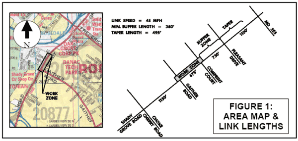
A queue length analysis using field data collected (including a.m. peak hour traffic volumes and signal timings) also was performed in order to determine how far upstream of the work zone should the analysis extend. Based on this queue length analysis, the analysts determined that the work zone analysis should extend at least 7,000 feet upstream of Gaither Road, the southernmost point of the lane closure. The recommended work zone analysis area is shown on Figure 66. No detour routes have been included in the analysis area as there are no nearby parallel routes. Also as shown by the figure, the study network extends from Choke Cherry Road to the EB I-370 On-ramp.
In addition to the identification of the size of the study area and the scope of the analysis, the analysts at this stage must identify the data needs required to model the alternatives. Data sources can include road geometry, signal timing plans, traffic demands, capacities, travel times, and queues. The following summarizes the data inputs to develop and run the Synchro/SimTraffic models:
Figure 66. Shady Grove Road –Extent of Analysis
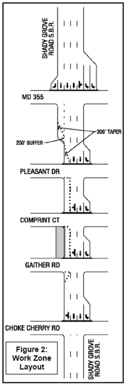
(Source: Maryland State Highway Administration, 2008.)
Field Data Collection Considerations
Although not specified in this case study, there are certain factors that should be considered when collecting volume and demand information from the field. First, the field analysts must consider the time periods when best to collect the data. For instance, if the work zone is to be completed during peak or off-peak periods, the time period for field data collection should be customized for when the work zone is planned/programmed to be active.
Second, analysts should consider the variations of daily traffic flow patterns and how this phenomenon can be captured through the data collection. In order to replicate the stochastic nature of traffic, the field analysts should plan to capture data through several days and/or multiple time periods. They should also consider the type of travel days (weekdays versus weekends) when data should be collected.
The next step of the MOTAA is to develop the existing conditions model with the appropriate geometry, traffic controls, demands, and capacities using the information from the data collection effort described in Step 5A. As previously mentioned, the MD SHA has coded most arterials in the State using Synchro. Typically, these can be used for the existing conditions model granted the study area already has been coded in these pre-developed networks. However, there were no existing Synchro models developed for the Shady Grove study area. Therefore, a new model was coded using information from the data collection effort.
Network coding of the study area was validated by field observations and supplied data by local, regional, and state agencies. The analysis time period also was determined from field observed traffic conditions. According to a fatal flaw analysis of these observations, the existing congestion level along Shady Grove Road in both the a.m. and p.m. peak periods would make the lane closure during these time periods infeasible. Therefore, the agency decided that construction needed to be conducted during the midday. As a result, all model scenarios were analyzed during the midday peak. Hence, only midday peak period signal timing, volume, and traffic conditions data were relevant for model development.
After the development of an existing conditions model, the following step in the MOTAA process is model calibration. Calibration ensures that the operational performance of the model replicates field observed conditions. In the Shady Grove case study, the model was calibrated using peak hour factors, truck percentages, and lane utilization factors. Once calibrated to these factors, the model was validated to reflect the queue conditions and travel times observed on the field.
In order to obtain model outputs for the base condition preconstruction, five SimTraffic simulation runs of the existing conditions model were performed. The model outputs extracted included control delay, LOS, and travel time. The existing conditions model outputs are shown in Table 91.
Additional Considerations for Model Calibration
There were few details provided regarding the model calibration procedure used in this case study. Chapter 4 of this document provides further details on recommended calibration procedures for models developed using traffic signal optimization tools. The following also lists some of the important components of a model calibration process:
The next stage of the MOTAA is the work zone base conditions model development. If an existing conditions model was developed it can typically be modified to develop the work zone base conditions and alternative models. The first work zone alternative or work zone base scenario for this case study is the right lane closure in the southbound direction of Shady Grove Road during the midday peak. As shown on the work zone layout on Figure 66, the lane closure occurs between the intersections of Shady Grove and Gaither Road and Comprint Court. The work zone layout also includes a buffer length of 360 feet and a merging taper of 495 feet. The main changes between the existing conditions model and this work zone scenario include the geometric changes needed to incorporate the lane closure into the network. No changes were made in the O-D data and traffic volumes.
No work zone base conditions model calibration was conducted for this case study.
Work Zone Base Conditions Model Calibration Options
As specified in Chapter 4 of this document, work zone model calibration includes the calibration of work zone capacity and performance measures. Work zone model capacity and performance measures, such as queue, travel time, delay, and speeds, can be calibrated to field data and or prior experiences (from similarly implemented work zone projects). Additionally, work zone base conditions calibration also entails that the analyst evaluate and identify the appropriate modeling parameters to use based on prior experiences modeling or analyzing work zones of similar types. Such observations and measures will aid the analyst in the work zone calibration process.
The alternatives analysis step typically involves two stages: 1) development of models to capture the scenarios or alternatives; and 2) description of how these models were run, the outputs extracted, and analysis of the results. In this case study, model simulation results were first extracted from the developed work zone base case scenario prior to the development of the second work zone alternative.
As previously mentioned, the work zone base case scenario model was run before the development of the second work zone alternative, the weekend work zone model scenario. Similar to the existing conditions model, five SimTraffic simulations were run for the work zone base case. The measures extracted from these model runs are featured in Table 92.
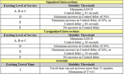
The next step is to determine whether the work zone base model results meet the MD SHA mobility thresholds for arterials shown on Figure 67. The intersections with performance measures shown bolded in red in Table 92 have failed to meet the mobility thresholds. For instance, the Gaither Road intersection that had a control delay of 34.4 seconds and an LOS C during the existing conditions model (as shown in Table 91), must meet the mobility threshold of a maximum of LOS D and control delay that must be less than or equal to 45 seconds in the work zone conditions model. Since the level of service of this intersection worsened to an LOS F and increased to a control delay greater than 45 seconds, the intersection failed to meet the mobility threshold. The results indicated another work zone alternative or mitigation measures should be considered.
Because of the nature of the work, the agency did not think it was feasible to consider other alternatives, such as reversible lanes or full lane closures, which would cause greater mobility impacts and require a greater amount of resources. Therefore, the agency decided that only work zone alternatives that involved lane closures during the off-peak hours would be feasible. The second alternative, therefore, considered was weekend construction.
Figure 67. MD SHA Work Zone Analysis Guide Mobility Thresholds for Arterials
In order to develop the weekend work zone model, weekend data such as weekend peak hour counts needed to be collected. The weekend peak hour was assumed to occur on Saturday midday. The existing conditions and work zone base conditions model were modified to create this work zone alternative by revising the model volumes and signal timings to reflect the weekend conditions. All lane configurations and geometric network features remained the same.
Similar to the existing and work zone base models, five simulations also were run for the weekend work zone scenario. Table 93 shows the existing conditions performance measures and the weekend work zone model results in parentheses. Based on the results shown in this table, all of the intersections met the mobility thresholds. The overall corridor also met the travel time thresholds.
The final stage of the MOTAA is the recommendation of the preferred alternative. The decision criteria for the MD SHA case studies are based on whether the alternative meets the mobility thresholds. Based on the results shown in Table 93, the weekend work zone scenario is the recommended alternative.
Decision Framework Options
This case study’s decision-making framework is based primarily on the mobility measures extracted from the Synchro/SimTraffic models. Although these results may be used in choosing a preferred scenario, there also are additional factors that an agency may want to consider when evaluating and comparing the alternatives. These factors are described in further detail in Chapter 7 of this document. A decision-making framework that incorporates these factors, as well as the mobility measures, can then be used to develop a methodology or criteria that can be used to compare the alternatives and choose a preferred option. Chapter 5 of this document features several different decision framework options that can fit projects of different complexities and resources.
This case study is based on the I-465 west leg reconstruction project in Indianapolis, Indiana as detailed in HCM 2010 Manual, Volume 4, Case Study 6. (Highway Capacity Manual 2010 (HCM 2010), Volume 4: Applications Guide. Transportation Research Board, National Research Council, Washington, D.C. Accessed January 11, 2012.) The reconstruction along I-465 is about nine miles in length with a total of eight interchanges. Figure 68 provides an overview of the location and extents of the project.
This section provides an overview of the analysis methodology employed in evaluating the mobility impacts of the interchange reconstruction on one segment of the I-465 west leg reconstruction, the Rockville Road Interchange Reconstruction Project, shown in Figure 69.
Figure 68. I-465 West Leg Reconstruction, Indianapolis Overview
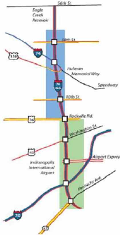
(Source: Transportation Research Board, 2010.)
Figure 69. I-465 Case Study Rockville Road Interchange Reconstruction Study Area
(Source: Transportation Research Board, 2010.)
The main purpose of this case study as featured in HCM 2010, Volume IV was to demonstrate the systemwide analysis of freeway and arterial traffic together with various lane closure options through the use of traffic analysis tools and procedures. Because this case study was featured in HCM 2010 for a specific purpose, the agency’s goals and objectives at the time of the reconstruction were not clearly stated. However, an example goal of an agency conducting a similar effort may be to find the optimal lane closure configuration that can minimize the mobility impacts of the work zone without sacrificing construction schedule/duration.
Tradeoffs typically exist between the duration of construction and the level of closures. While lane closures can improve construction duration, the mobility impacts can generate huge disbenefits to motorists, neighborhoods, and businesses. The objective of the modeling analysis, therefore, could be to use the performance measures generated from the analysis to compare work zone configuration options and determine the optimal alternative for the interchange reconstruction.
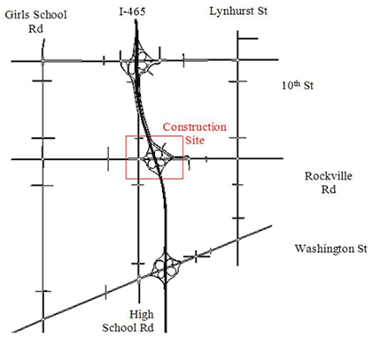
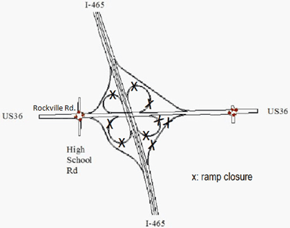
In addition, to identifying the goals and objectives of the project, another key part of this stage of the MOTAA is to identify the scope and extents of the analysis. The analysis extent covers the area shown in Figure 70. In this case study, five on- and off-ramps of the Rockville Road interchange will be closed during construction. These include four loop ramps and the I-465 NB to Rockville Road EB off-ramp. Ramps that are closed are marked by an “x” as shown in Figure 70.
Figure 70. Rockville Road/U.S. 36 Interchange Ramp Closures
(Source: Transportation Research Board, 2010.)
After defining the goals and objectives of the project, the next step in an MOTAA is to establish the measures of effectiveness and/or thresholds that would be used to evaluate and compare the different work zone alternatives. For this case study the mobility performance measures chosen include average speed and average number of vehicles present in the network, as well as average and cumulative network delays. Another measure that was considered in this case study was construction duration.
The next stage of the MOTAA process is to determine the type of analysis tool to be used and the justification for that selection. In this case study, PARAMICS was selected as the simulation tool and Synchro was used to develop signal timing plans. According to the HCM 2010 write-up of this case study, HCM methodologies are not robust enough to generate results and performance measures that could aid in identifying the lane closure alternative that minimizes impacts while improving construction duration. Therefore, the combination of traffic signal optimization and microsimulation analysis tools was used.
Additionally, the analysts wanted to report measures at different levels of analysis (link-, facility-, and systemwide). While operational measures can be generated using HCM methodologies at a link-specific and intersection level, HCM is not suitable for reporting measures at a systemwide level such as for the interchange as a whole. On the other hand, microsimulation has the ability to conduct an operational analysis at link-specific, intersection, multi-facility, and systemwide levels. In the Rockville Road Interchange case study, microsimulation enables the analyst to conduct the impact analysis and generate performance measures for various facility sizes such as for the entire interchange, specific facilities (freeways, ramps, or arterials), or individual links. Additionally, microsimulation tools are useful for analyzing the temporal fluctuations of traffic operations. The combination of microsimulation and traffic signal optimization tools offered the analysts the capabilities required in order to generate the mobility measures identified in Step 2.
Analysis Tool Selection Options
This case study’s tool selection process focused on the tools’ capabilities to capture certain measures of mobility and the scope of the analysis. There are additional factors that an analyst can consider when selecting the appropriate analysis tool. Chapter 3 of this document describes these various factors in greater detail. The recommended factors for identifying the appropriate modeling approach include:
After determining the MOEs and the analysis tool, the next stage of an MOTAA process is the identification of work zone alternatives. As previously mentioned in Step 1 – Project Scope, lane closures on Rockville Road are flexible based on the mobility impacts of the work zone. As a result, the objective of the analysis is to evaluate various lane closure alternatives at Rockville Road and determine their impacts on mobility and construction duration. The three-lane closure scenarios at Rockville Road included the following:
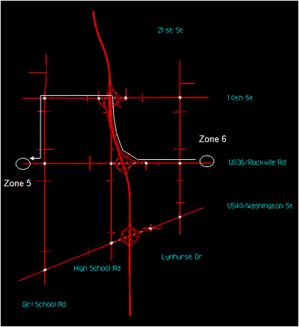
During this stage of the modeling development and analysis, the analysts should define the scope of the analysis and identify the data needed for the calibration and modeling analysis effort. Part of project scoping is defining the study area that will be evaluated during the analysis. In this case study, the analysis covers the area consisting of the entire Rockville Road Interchange and the two intersections at the ramp termini on both sides of the interchange, as shown in Figure 71.
Extent of Analysis Considerations
Although the particular focus of this analysis is on the Rockville Road Interchange and two signalized intersections at the ramp termini, the extent of the analysis can be extended to one to two interchanges both north and south of the study area as well as the parallel arterials on either side of the interstate. Extending the area to be analyzed will enable the analyst to identify potential alternative routes and assess the mobility impacts of the Rockville Road ramp closures not only on Rockville Road, but also on adjacent interchanges and parallel arterials. An example of potential model size for analysis is shown in Figure 71.
In addition to determining the scope of the analysis, at this stage of the MOTAA the analyst also must identify the data inputs and assumptions needed to model the scenarios. Data collection efforts for microsimulation models typically require data on road geometry, controls, traffic demands, capacities, travel times, and queues. The baseline model of this case study will be based on 2006 existing conditions data. The following summarizes the data collection effort for the interchange reconstruction scenarios:
Demand Data and Analysis Period Considerations
For this case study, a 24-hour demand profile was constructed in order to evaluate travel conditions before, after, and during the peak periods. However, due to resource requirements and simulation processing and run times needed for microsimulation models, a 24-hour analysis period is atypical for this type of tool. Such models would typically be run for specific time periods such as a three- to four-hour window (i.e., peak period or off-peak). An example AM peak period O-D table for the study area network is shown in Figure 73.
The next step of the MOTAA is to develop the existing conditions model with the appropriate geometry, traffic controls, demands, and capacities using the information from the data collection effort, specified in Step 5A.
Error Checking in Model Development
Although not specified in this case study, during model development, the analyst should perform error checks to identify and correct any model coding and signal timing errors. The analyst can check the model network geometries and traffic control operations against existing plans or engineering drawings obtained in Step 5A.
Figure 71. Rockville Road Case Study – Example Model Extents
(Source: Transportation Research Board, 2010.)
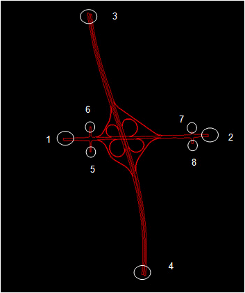
Figure 72. Rockville Road Interchange Case Study – Locations of Zones for O-D Table
(Source: Transportation Research Board, 2010.)
Figure 73. Rockville Road Interchange Case Study – Example AM Peak Period Existing Conditions O-D Table
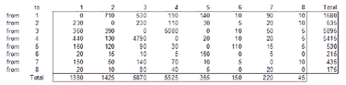
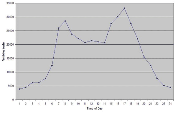
Figure 74. Rockville Road Interchange – Existing Conditions Model 24-Hour Demand Profile
(Source: Transportation Research Board, 2010.)
After the development of an existing conditions model, the following step in an MOTAA process is model calibration. Model calibration ensures that the operational performance of the model best reflects field observed conditions. The existing conditions model’s volumes and speeds were validated with the information obtained during the data collection effort outlined in Step 5A.
Additional Considerations for Model Calibration
The model calibration effort for the Rockville Road Interchange Reconstruction was not described in great detail in HCM 2010. However, for additional guidance on model calibration, refer to Chapter 4 of this document. Additionally, the following lists the factors typically involved in a model calibration process:
The next step in the MOTAA process is the development of the work zone base conditions model. If an existing conditions model was developed it can typically be modified to develop the work zone base conditions model, as well as the alternatives analysis scenarios. In this case study, there was no work zone base conditions model developed. Since no work zone base conditions model was developed, there was no need for a work zone base conditions model calibration.
Work Zone Base Conditions Model Calibration Options
As specified in Chapter 4 of this document, work zone model calibration includes the calibration of work zone capacity and performance measures. Work zone model capacity and performance measures, such as queue, travel time, delay, and speeds, can be calibrated to field data and or prior experiences (from similarly implemented work zone projects). Additionally, work zone base conditions calibration also entails that the analyst evaluate and identify the appropriate modeling parameters to use based on prior experiences modeling or analyzing work zones of similar types. Such observations and measures will aid the analyst in the work zone calibration process.
The alternatives analysis step involves two stages: 1) the development of models to capture the scenarios or alternatives; and 2) the methodology that describes how the models were run, the process for extracting outputs from the model, and the analysis of the results.
This case study featured three alternative scenarios, as described in Step 4. The following three models were coded by modifying the 2006 existing conditions model.
The final steps of the MOTAA are to run the work zone alternative models using the selected traffic analysis tool and to extract the model outputs needed to generate the MOEs established in Step 3. The following summarizes the resulting measures of effectiveness generated for each model scenario:
Figure 75. Rockville Road Interchange – Average Network Speed
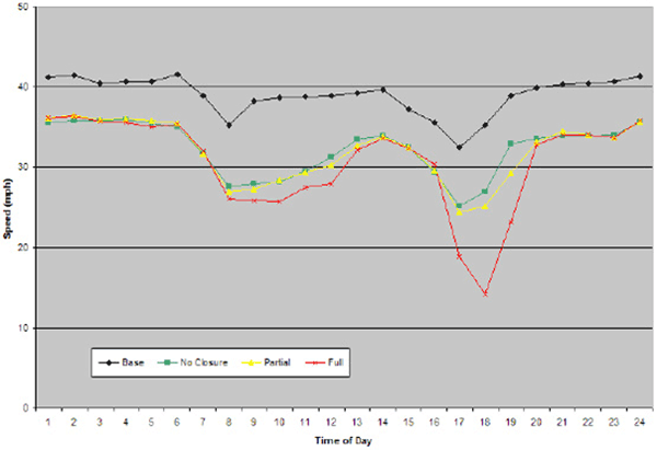
(Source: Transportation Research Board, 2010.)
Figure 76. Rockville Road Interchange – Average Number of Vehicles
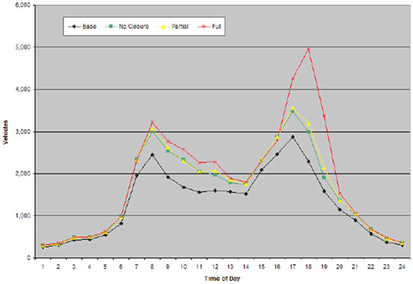
(Source: Transportation Research Board, 2010.)
Figure 77. Rockville Road Interchange – Average Network Delays
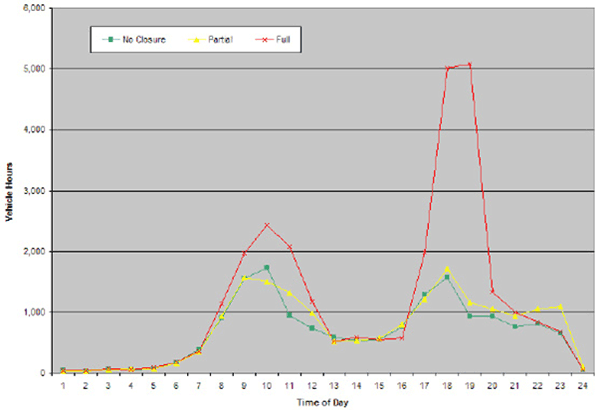
(Source: Transportation Research Board, 2010.)
Figure 78. Rockville Road Interchange – Cumulative Network Delays
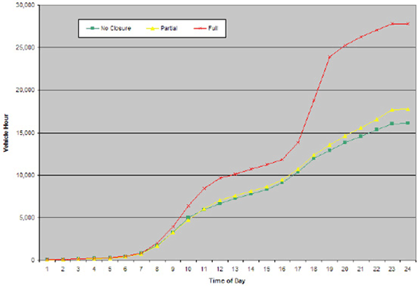
(Source: Transportation Research Board, 2010.)
Figure 79. Rockville Road Interchange Reconstruction – Cumulative Network Delays during the Construction Period
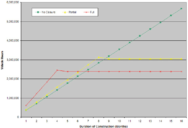
(Source: Transportation Research Board, 2010.)
In the HCM 2010 Manual, the case study does not indicate which of the three alternatives should be recommended for implementation, nor how the alternatives analysis results can be used to select a preferred construction scenario.
Decision-Framework Options
Although this case study does not feature a decision-framework, the following example shown in Figure 80 illustrates an example showing how the alternatives analysis results can be used to develop decision-making criteria for identifying a preferred alternative. There are several decision-making frameworks that can be used to evaluate and choose among different work zone alternatives. Several of these frameworks are described in further detail in Chapter 5.
In the following example shown in Figure 80, a hypothetical 100-point scale was developed to score the various alternatives against a set of criteria. The table shows the alternatives’ mobility measures extracted from the alternatives analysis results. It also includes assumed values for measures such as road user costs, construction duration, and safety for each alternative.
In some instances, the measure shown in Figure 80 refers to evening peak traffic conditions. In order to report these measures using this specific timeframe, the values associated with 4:00 p.m. to 7:00 p.m. from the 24-hour alternatives analysis results were averaged. Each alternative’s performance measures were then compared against a set of criteria, which determines how many points should be allotted to each alternative based on the values of each MOE. According to the results of this hypothetical scoring technique, the No Closure alternative (highlighted in green) scored the highest of the three alternatives.
Figure 80. I-465 West Leg, Rockville Road Interchange Reconstruction Decision Framework Example
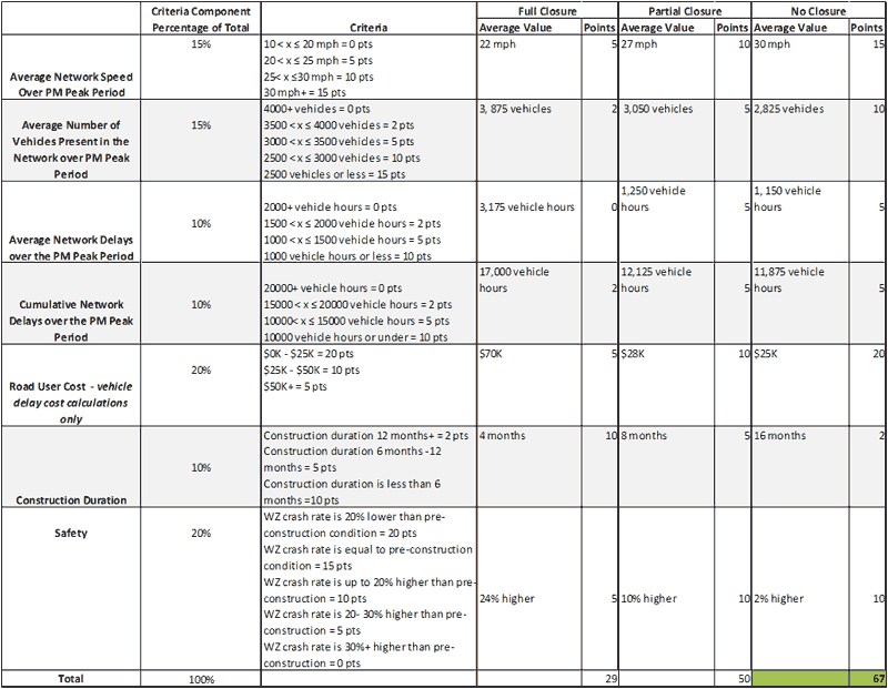
This case study describes the process to evaluate potential maintenance of traffic detour routes and a potential full closure option during the planning phase of the Cleveland Innerbelt Project in 2004 for the Ohio DOT. (Bugess & Nipple, Inc. The Cleveland Innerbelt Project. Ohio Department of Transportation, 2004.)
The Cleveland Innerbelt is a high capacity, limited-access interstate highway extending from Cleveland’s Tremont neighborhood on the west side of the Cuyahoga River, across the Cuyahoga Valley, around the southern and eastern edges of downtown to the City’s lakefront district at Burke Lakefront Airport. The Innerbelt includes portions of I-71 and I-90, and connects to I-77, I-490, SR 2, and SR 176, as shown in Figure 81.
A key component of the Innerbelt Freeway is the Central Viaduct Bridge, shown in Figure 82. The Central Viaduct Bridge is a primary river crossing, moving Interstate traffic from the south (I-71) and west (I-90) across the Cuyahoga River to the downtown distribution system of the Central Interchange and further east to the Innerbelt Trench. The near mile-long Central Viaduct Bridge is the critical link along this section of I-90 carrying over 130,000 vehicles per day.
Figure 81. Cleveland Innerbelt Project
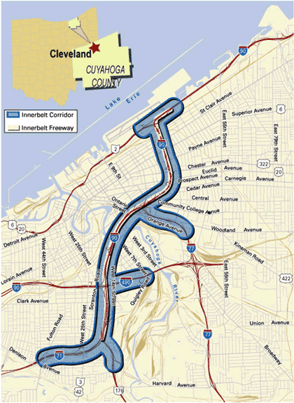
(Source: Bugess & Nipple, Inc., 2004.)
Figure 82. Cleveland Innerbelt Corridor Sections
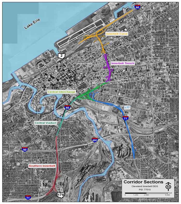
(Source: Bugess & Nipple, Inc., 2004.)
The daily recurring congestion presents a tremendous challenge for maintenance of traffic during construction. The entire length of the Innerbelt Freeway lacks adequate shoulders on which to perform or stage construction work. Further, Ohio DOT maintenance of traffic policies discourage long-term lane closures on this portion of I-90 due to high traffic demand and existing poor levels of service. As such, there is need to plan for a systematic phasing of the improvements, such that traffic can be maintained to the greatest extent practical.
In accordance with Ohio DOT Policy Number 516-003(P) Traffic Management in Work Zones: Interstate and Other Freeways, Ohio DOT District 12 has developed a Permitted Lane Closure Map (PLCM) (shown in Figure 83) that specifies how many lanes must remain open during what time periods in order to minimize construction-related congestion and delay. (Ohio Department of Transportation. Traffic Management in Work Zones: Interstate and Other Freeways. Accessed January 11, 2012.) The sequencing of construction needed to be programmed to minimize traffic delays throughout the corridor. Within construction areas, it was planned that traffic control measures using standard practices would be used.
During the Planning Phase of this project, a Cleveland Innerbelt MOT Strategic Plan was developed to assist in quantifying the potential impacts of MOT activities on the study area and to help identify additional projects that may need to be completed as part of the overall implementation strategy to help mitigate these impacts. To support this effort, the primary and secondary maintenance of traffic routes that may be utilized by motorists during construction, whether officially signed or not, needed to be identified.
The project also hosted an Accelerated Construction Technology Transfer (ACTT) review during the planning process. One of the issues raised at this ACTT review was the potential to accelerate the replacement of the Central Viaduct by initiating a full closure of the bridge and, thus, accommodating the full replacement of the structure on the existing alignment. The impact of this full closure also needed to be determined before additional project resources would be utilized to pursue it. As such, a “red flag”-level analysis was undertaken for this alternative.
Figure 83. Ohio DOT Permitted Lane Closure Map (PLCM)
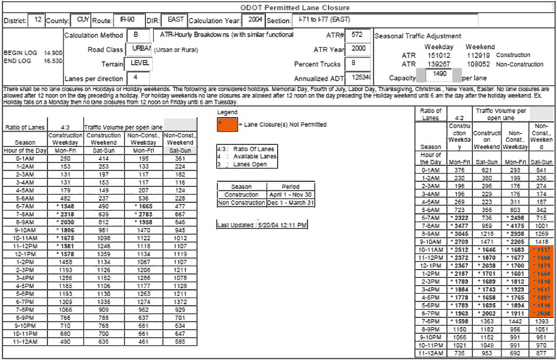
The first step in an MOTAA is to define the scope, goals, and objectives of the analysis. Based on the requirements of this analysis, it was necessary to identify primary and secondary maintenance of traffic corridors and to determine the feasibility of implementing a full closure of the Central Viaduct Bridge. A vital goal for controlling traffic through and around the projected construction work zones was to minimize the disruption of normal traffic flow and maintain reasonable access to all properties near the construction areas.
After defining the goals and objectives of the project, the next step in an MOTAA is to establish the measures of effectiveness and/or thresholds that would be used to evaluate and compare the different work zone alternatives. For this case study, the mobility measures of effectiveness (MOE) selected included percent increase or decrease in traffic and volume/capacity (v/c) ratio.
The next stage of the MOTAA process is to determine the type of analysis tool to be used and the justification for that selection. In this case study, TRANPLAN, the regional travel demand model, was chosen as the operational model platform to simulate traffic assignments due to its ease of use, ready access, and ability to generate the measures of effectiveness determined in Step 2. Factors that impacted the decision to utilize a travel demand model as the analysis tool are as follows:
Analysis Tool Selection Options
There are additional factors that an analyst can consider when selecting the appropriate analysis tool. Section 3 of this document describes these various factors in greater detail. The recommended factors for identifying the appropriate modeling approach include:
After determining the MOEs and the analysis tool, the next stage of an MOTAA process is the identification of work zone alternatives. As a baseline for comparison, the existing conditions model would be utilized. In addition, two additional models will be utilized to determine potential impacts.
During this stage of the modeling development and analysis, the analysts should define the objectives of the analysis and identify the data needed for the calibration and modeling analysis effort. This step was unnecessary as part of this analysis. Earlier efforts within the project to make improvements to the fidelity of the route assignment component of the model through splitting zones and adding a parking allocation model already had been completed. Further, the validation of the growth projections in conjunction with the Neighborhood Planning Committee also removed the need for additional data checks.
The next step of the MOTAA is to develop the existing conditions model with the appropriate geometry, traffic controls, demands, and capacities using the information from the data collection effort and the preliminary analysis. As discussed above, refinements to the existing model already had been undertaken as part of a parallel process during the project.
The model calibration was conducted through the Neighborhood Planning Committee growth projection validation process. The validation was mainly focused on v/c ratio and traffic volumes on freeways and major arterials. For traffic volume validation, the acceptable threshold between modeled volumes and field counts on major freeways and arterials were within 10 percent.
Once the existing conditions model has been developed and calibrated, it can then be modified for use during the work zone base conditions model development and calibration, as well as during the alternatives analysis stage. In this case study, there was no work zone base conditions model developed. The scenarios identified in Step 4 were considered as alternatives. Therefore, all runs would be compared to existing conditions, as there were no work zone base conditions.
No work zone calibration procedure was specified for this case study.
Work Zone Base Conditions Model Calibration Options
As specified in Chapter 4 of this document, work zone model calibration includes the calibration of work zone capacity and performance measures. Work zone model capacity and performance measures such as queue, travel time, delay, and speeds can be calibrated to field data and or prior experiences (from similarly implemented work zone projects). Additionally, work zone base conditions calibration also entails that the analyst evaluate and identify the appropriate modeling parameters to use based on prior experiences modeling or analyzing work zones of similar types. Such observations and measures will aid the analyst in the work zone calibration process.
The alternatives analysis step involves two stages: 1) development of models to capture the scenarios or alternatives; and 2) description of how these models were run, the outputs extracted, and analysis of the results.
The analysts started with the existing conditions model and adjusted the roadway network to replicate each of the scenarios identified in Step 4. The adjustments included geometric configurations (e.g., number of lanes), capacities, and link length change to match work zone area. The model was run for the a.m. peak period only.
The final step of the MOTAA is to run the work zone alternative models and evaluate the mobility performance measures extracted from the model results. As previously mentioned, the analysts used percent increase or decrease in traffic and v/c ratio as MOEs. These results were then thematically displayed on a series of graphics showing the impact of each of the alternatives. Figures 84 and 85 show the v/c ratio thematic plots for Alternative 1 (full closure) and Alternative 2 (partial closure), respectively.
Figure 84. Cleveland Innerbelt Study: V/C Ratio Thematic Map
(Alternative 1 – Full Closure)
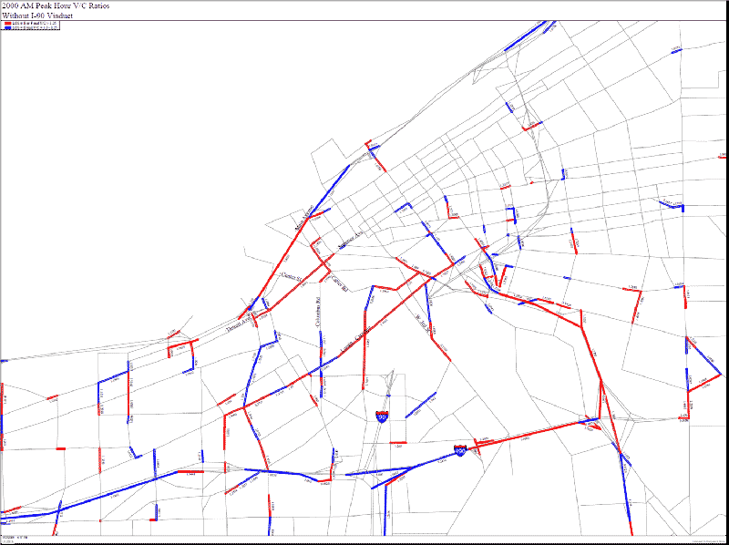
(Source: Bugess & Nipple, Inc., 2004.)
Figure 85. Cleveland Innerbelt Study: V/C Ratio Thematic Map
(Alternative 2 – Partial Closure)
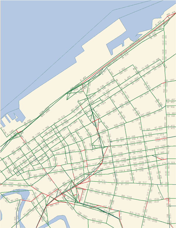
(Source: Bugess & Nipple, Inc., 2004.)
After obtaining the model output and mobility performance measures through the modeling analysis, the next stage of the MOTAA process is the application of a decision-making framework or criteria for evaluating and identifying the preferred alternative.
A red flag analysis of the concept of a full closure of the Central Viaduct Bridge (Alternative 1) was conducted. The thematic map (Figure 85) showed that by completely removing this critical link from the highway network, the potential detour routes were overwhelmed by diverting traffic. This would have had a critical impact on the ability to provide access to and from the CBD of Cleveland from both the south and west. As such, this alternative construction technique was removed from further consideration.
Alternative 2 was recommended based on a combination of engineering judgment and public involvement with key stakeholders to aid in the development of the plan. The thematic mapping results from the travel demand model were utilized to show where potential traffic diversion routes could be expected. This information was shared with key stakeholders in a charrette setting along with additional information regarding location of key community resources, adjacent land use, noise susceptible properties, minority populations, low-income populations, zoning, historic resources, etc. Working with the community in a facilitated environment, routes were identified as either primary or secondary maintenance of traffic routes (see Figure 86). As the project moves forward, as much traffic as can safely be accommodated should remain on the freeway. When traffic must be diverted to the arterial street system it should be focused onto the primary maintenance of traffic routes and discouraged from using the secondary routes. To accomplish this, the MOT Strategic Plan identified additional projects or concepts that would be added to the overall scope of the project to support the needs of accommodating this approach. Examples of these types of recommendations include:
Decision Framework Options
The analysts in this case study used the mobility MOEs that were output by the modeling analysis to support an interactive process with the community for identifying primary and secondary maintenance of traffic corridors. In this instance, mobility measures were only a piece of the overall decision-making framework. As such, a formalized decision-making framework was determined to be detrimental to the process of building consensus with the stakeholders.
Figure 86. Cleveland Innerbelt Study: Maintenance of Traffic Corridors Map
(Source: Bugess & Nipple, Inc., 2004.)
This case study describes the process used by Kremer, et al. (2000) to evaluate several construction staging proposals for the project improvements completed along the I-80 eastbound corridor in Saddle Brook, Bergen County, New Jersey in 1999. (Kremer, P.F., A.W. Kotchi, A.J. DeJohn, and K.B. Winslow. The Use of Operational Models to Evaluate Construction Staging Plans, A Case Study. Parsons Brinckerhoff, Inc., 2001.) The improvements occurred between Interchange 62 and 64 along I-80 and included roadway widening, noise wall erection, and bridge deck replacement. The improvements were necessary as I-80, a key commuter route for the region, was in great need of additional capacity. The work zone alternatives analysis was conducted in order to determine how to perform the improvements necessary with the least possible impacts to road users.
Figure 87 depicts the existing conditions or preconstruction configuration of I-80 eastbound. At one end of the study area, I-80 eastbound consisted of five lanes approaching a Collector-Distributor (C-D) Road that provided access to the Garden State Parkway and Saddle River Road. The section then became a four-lane section that eventually turned into a split configuration consisting of two express lanes and two local lanes. The express lanes provided direct access to the New Jersey Turnpike and George Washington Bridge. The local lanes provided access to all interchanges in between.
The following subsections describe the work zone alternatives analysis procedure applied and documented in a Transportation Research Board paper by Kremer, et al. (2000) in evaluating the construction staging alternatives for the I-80 project improvements completed in 1999. (Kremer, P.F., A.W. Kotchi, A.J. DeJohn, and K.B. Winslow. The Use of Operational Models to Evaluate Construction Staging Plans, A Case Study. Parsons Brinckerhoff, Inc., 2001.) The purpose of the case study analysis was to present an alternative approach to the typical construction staging analysis. The authors described the typical construction staging analysis as a procedure that involved identifying critical demand and designing staging plans to ensure that sufficient capacity exists in the construction zone to meet that measured demand. The authors noted that this approach treats demand as isolated points instead of viewing flows as a system. Examining traffic flow at a systemwide level would ensure that the analysis accounted for both upstream and downstream conditions. The process they recommended offers a four-step approach that includes the following:
The authors’ four-step process parallels many of the concepts incorporated into the recommended MOTAA methodology described in Chapters 2 and 4 of this document. However, for the purpose of this guide, the authors’ proposed process will be tailored to fit the step-by-step methodology described in Chapter 4.
The first step in an MOTAA is to define the goals and objectives of the analysis. This also corresponds with the authors’ first stage of their four-step process. In this case study, I-80 is a principal east-west travel route in New Jersey, providing vital linkages for travelers between local destinations within the State, as well as interstate between New York, New England, New Jersey, and Pennsylvania. The construction work zone was, therefore, located in one of the most heavily traveled sections of I-80 in the State. I-80 already is severely congested during the peak period and any other disruption and reduction in capacity would severely impede mobility. The goal of the project was, therefore, to determine the construction staging option that could minimize the disruption experienced by motorists through accommodating current traffic demand without a significant spatial or temporal shift.
After defining the goals and objectives of the project, the next step in an MOTAA is to establish the measures of effectiveness and/or thresholds that would be used to evaluate and compare the different work zone alternatives. For this case study the MOEs chosen included average speed, travel time, queue length, and vehicle throughput.
The next stage of the MOTAA process is to determine the type of analysis tool to be used and the justification for that selection. In this case study, INTEGRATION was chosen as the operational model platform to simulate traffic operations due to its ease of use and ability to generate the measures of effectiveness determined in Step 2. A mesoscopic model was chosen because of its ability to allow users to test various scenarios and generate a more accurate range of performance measures for comparison among alternative design and operational scenarios as compared to travel demand models. It also was chosen because of its ability to generate various measures of effectiveness, including travel times by vehicle or link type, queue length, duration, and visual observations of queue formation and dissipation.
Analysis Tool Selection Options
There are additional factors that an analyst can consider when selecting the appropriate analysis tool. Chapter 3 of this document describes these various factors in greater detail. The recommended factors for identifying the appropriate modeling approach include:
For this case study, the analyst chose a tool that was consistent with most of these factors. A mesoscopic simulation software package such as INTEGRATION was chosen based on the data needs, analysis goals and objectives, the transportation management plan, and performance measures required for the project.
Figure 87. I-80 Eastbound Existing Conditions
(Source: Kremer, Kotchi, DeJohn, and Winslow, 2001.)
After determining the MOEs and the analysis tool, the next stage of an MOTAA process is the identification of work zone alternatives. Aside from the existing conditions scenarios described in the Project Background portion of this section, the two alternatives/construction staging scenarios compared and evaluated in this case study includes:
During this stage of the modeling development and analysis, the analysts should define the objectives of the analysis and identify the data needed for the calibration and modeling analysis effort. Data collection efforts for microsimulation models typically require data on road geometry, controls, traffic demands, capacities, travel times, and queues. This step would correspond with the second stage of the four-step process identified by the authors.
The scope of this case study was to design and evaluate the construction staging area along I-80 eastbound between Interchanges 62 and 64. As previously mentioned, the objective of the analysis effort is to conduct the construction effort with minimal disruption to mobility. The analysis effort evaluated the study area during the a.m. peak period between 6:30 a.m. and 9:00 a.m.
Figure 88. I-80 Eastbound Contract Staging Plan
(Source: Kremer, Kotchi, DeJohn, and Winslow, 2001.)
Figure 89. I-80 Eastbound Contractor Staging Alternative
(Three-Lane Staging Plan)
(Source: Kremer, Kotchi, DeJohn, and Winslow, 2001.)
The data collection effort included:
A preliminary traffic engineering evaluation also was conducted to determine the roadway capacity and throughput in the study area. The preliminary traffic engineering evaluation included:
The next step of the MOTAA is to develop the existing conditions model with the appropriate geometry, traffic controls, demands, and capacities using the information from the data collection effort and the preliminary analysis. The process used in the case study for network coding and error checks included:
The model calibration criteria consisted of three sources of existing conditions data: traffic counts, average travel speeds, and queuing observations. The calibration was determined to be within acceptable limits. Results of the calibration effort were not shared in the document.
Additional Considerations for Model Calibration
For this case study, the criteria measures used to compare model behavior with field observations were established. However, there are several other considerations involved in the model calibration process, including:
Once the existing conditions model has been developed and calibrated, it can then be modified for use during the work zone base conditions model development and calibration, as well as during the alternatives analysis stage. In this case study, there was no work zone base conditions model developed. The analysts assumed the same demand levels for all three scenarios (existing conditions, contract staging plan, and alternative staging plan). No work zone calibration procedure was specified for this case study.
Work Zone Base Conditions Model Calibration Options
As specified in Chapter 4 of this document, work zone model calibration includes the calibration of work zone capacity and performance measures. Work zone model capacity and performance measures such as queue, travel time, delay, and speeds can be calibrated to field data and or prior experiences (from similarly implemented work zone projects). Additionally, work zone base conditions calibration also entails that the analyst evaluate and identify the appropriate modeling parameters to use based on prior experiences modeling or analyzing work zones of similar types. Such observations and measures will aid the analyst in the work zone calibration process.
For many work zone projects, the absence of reliable work zone conditions data to calibrate has caused many agencies to abandon a work zone base calibration effort. Instead, many of the same assumptions, parameters, and demands are consistent across the existing conditions and work zone conditions models. However, in reality, demands and driver behavior can be very different in a work zone versus a typical driving commute. While this case study does not provide a work zone base calibration effort, the following suggested procedure provides some recommendations and guidance on the calibration of a work zone base model.
1. Identifying Calibrations Measures and Thresholds
In the existing model calibration, field measures and/or observations such as volumes, speeds, queues, and bottlenecks were used to calibrate/validate model outputs. Since typically the work zone base condition model development occurs prior to project implementation, there is typically no field data to calibrate to. Analysts can, therefore, use similar measures for calibration/validation, but must rely on sources outside of field data. One example of a measure that can be used for work zone calibration is capacity during work zone conditions. Chapter 4 of this document describes how work zone capacity can be determined. Analysts can determine work zone capacity using any of the following methods/sources:
2. Parameter Adjustments
The next step entails the adjustment of model parameters until the model is able to replicate or reflect the conditions identified by the previous step. For instance, if the measure being used for the calibration procedure is capacity, the analyst can conduct a sensitivity analysis that will identify which combinations and values of model parameters are able to produce the expected capacity for the work zone. Some example model parameters that could be adjusted for work zone base calibration in INTEGRATION and other mesoscopic, as well as microscopic tools include:
Through a work zone base calibration procedure, the model can better reflect the expected capacity, demands, queues, and diversions that may occur as result of the work zone.
The alternatives analysis step involves two stages: 1) development of models to capture the scenarios or alternatives; and 2) description of how these models were run, the outputs extracted, and analysis of the results.
The analysts used the existing conditions model and adjusted it to develop the two alternatives analysis scenarios according to design plans. The analysts assumed that the same trip table, developed in Step 5A would be used for all three models: existing conditions, contract staging plan, and the contractor’s alternative staging plan. The analysis time period remained at 6:30-9:00 a.m., the morning peak period.
The final step of the MOTAA is to run the work zone alternative models and evaluate the performance measures extracted from the model results. As previously mentioned, the analysts used MOEs such as average speed, travel time, maximum queue length, and total vehicle throughput to evaluate and compare the work zone alternatives. The results of the analysis are shown in Figure 90.
Figure 90. I-80 Eastbound Alternatives Analysis Results
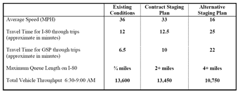
Determining the Number of Runs
One of the key steps in the alternative analysis is determining the appropriate number of models runs as specified earlier in Step 5C, existing conditions model calibration. Section 4.7 of this document also discussed how to determine the number of runs.
After obtaining the model output and mobility performance measures through the modeling analysis, the next stage of the MOTAA process is the application of a decision-making framework or criteria for evaluating and identifying the preferred alternative. In this case study, the authors chose the alternative that would generate the least amount of negative impacts on mobility along the corridor. According to the results shown in Figure 90, the Alternative Staging Plan would reduce the average travel speed by half, add 12 minutes to the travel time, and reduce throughput by about 3,000 vehicles as compared to the Contract Staging Plan. Therefore, the preferred alternative was the Contract Staging Plan.
Decision Framework Option/Example
The analysts in this case study chose the preferred alternative based on the mobility measures extracted from the modeling analysis. There are also additional factors outside of mobility measures that an agency may want to consider when evaluating the alternatives. These factors are described in further detail in Chapter 7 of this document. A decision-making framework that incorporates these factors, as well as the mobility measures from the simulation results can then be applied to compare the alternatives and choose a preferred option. Chapter 5 of this document feature several different decision-framework options that can fit projects of different complexities and resources.
The following illustrates the application of a decision-making framework, the Kepner-Tregoe (KT) Method, on the I-80 case study using the results from the alternatives analysis, as well as hypothetical values and assumptions for additional factors/measures. As discussed in Chapter 5 of this document, the KT Method involves the following steps:
Step1 – Prepare Decision Statement
The purpose of the decision analysis is to identify the most appropriate construction staging alternative for minimizing the project’s impacts on motorists and the community.
Step 2 – Define MUST and WANT objectives
As described in Chapter 5, MUST objectives include all mandatory requirements that the alternatives must meet. WANT objectives includes the desired measures that will be used to weigh/rank alternatives. The following example includes lists of objectives that serve as hypothetical examples for the purpose of demonstrating the KT Method. These objectives are not representative of established thresholds, requirements, or objectives set by the New Jersey DOT during the implementation of this I-80 project.
Decision Framework Option/Example
The list of MUST objectives include:
The WANT objectives include:
Step 3 – Assign weights to WANT objectives
In the next step of the KT method, weights are assigned to WANT objectives that reflect their relative importance in the decision-making process. A score of 1 indicates “least preferred” and a score of 10 indicates “most preferable.”
| No. | WANT Objective | Assigned Weight |
|---|---|---|
| 1 | Delay Costs | 10 |
| 2 | Vehicle Operating Costs | 8 |
| 3 | Construction Duration | 10 |
| 4 | Maintenance of Emergency Services | 6 |
Step 4 – Identify candidate MOT alternatives
The next step of the KT method is to identify the alternatives that will be compared and measured against the MUST and WANT objectives. The two work zone alternatives include the Contract Staging Plan and the Alternative Staging Plan.
Step 5 – Summarize the findings of the Work Zone Impact Assessment
The following table summarizes how the alternatives measure against the MUST objectives:
Decision Framework Option/Example
| MUST Objectives | Alternative Evaluation | |
|---|---|---|
| Contract Staging Plan | Alternative Staging Plan | |
| 1. Maintain at least two lanes of traffic within the work zone | Yes | Yes |
| 2. The maximum allowable queue length for any work zone duration is two miles | Yes | Yes |
| 3. Delays must be less than 30 minutes for complex projects | Yes | Yes |
The following table summarizes the impact assessment of the two work zone alternatives against the WANT objectives established in Step 2 of the KT Method:
| WANT Objectives | Alternative Evaluation | |
|---|---|---|
| Contract Staging Plan | Alternative Staging Plan | |
| 1. Delay costs | $39,400 | $54,700 |
| 2. Vehicle operating costs | $2,200 | $3,000 |
| 3. Construction duration | 16 months | 8 months |
| 4. Maintain emergency services/provisions (rated at poor, average, or good) | Good | Poor |
Step 6 – Evaluate Alternatives against MUST Objectives
The results shown on the MUST objectives table from the previous step indicate that both alternatives satisfy the mandatory requirement and/or thresholds. Therefore, both alternatives proceed to the next step.
Step 7 – Evaluate Alternatives against WANT Objectives
In this step of the KT Method, the alternatives are assigned a score (value between 1 and 10) against each WANT objective based on how well the alternative meets that objective. The following table shows the results of this evaluation:
| WANT Objectives | Alternative Score | |
|---|---|---|
| Contract Staging Plan | Alternative Staging Plan | |
| 1. Delay costs | 8 | 6 |
| 2. Vehicle operating costs | 9 | 7 |
| 3. Construction duration | 6 | 10 |
| 4. Maintain emergency services/provisions (rated at poor, average, or good) | 10 | 5 |
Step 8 – Calculate the Weighted Scores of the Alternatives
This step applies the weights established in Step 3 to the results of the alternatives evaluation for WANT objectives (previous step) in order to generate weighted scores for each alternative. For example, the weight of WANT objective “Delay costs” is 10. In order to calculate the weighted score, the weight of the objective is multiplied with the alternative score. For example, the weighted score for the Contract Staging Plan for the “Delay costs” objective is 10*8 or 80. The weighted scores for each alternative against each objective is shown on the following table:
| WANT Objectives | Weighted Alternative Score | |
|---|---|---|
| Contract Staging Plan | Alternative Staging Plan | |
| 1. Delay costs | 80 | 60 |
| 2. Vehicle operating costs | 72 | 56 |
| 3. Construction duration | 60 | 100 |
| 4. Maintain emergency services/provisions (rated at poor, average, or good) | 60 | 30 |
| Total weighted score | 272 | 246 |
As shown by the weighted score results, the Contract Staging Plan is the tentative choice.
Step 9 – Evaluate Adverse Consequences – Risk Assessment
This next step involves weighing the feasible alternatives against potential risks identified in the work zone impact assessment. The scores from this risk assessment is two-fold and incorporates considerations for the likelihood of the event occurring and the severity of the impact. The scores range from values of 1 through 10. When evaluating the probability of a risk or event occurring, a score of 1 indicates that the particular risk is unlikely to occur while 10 means most probable. When evaluating the severity of impact, a score of 1 indicates that the impact is “inconsequential” and a score of 10 indicates that the impact is “very severe.” The probability and the severity scores are multiplied in order to obtain the adverse consequence score by risk/event for each alternative. Once more, this example presents several hypothetical risk considerations. These risk considerations serve as examples for demonstrating the decision framework. These are not in any way representative of actual factors considered during the implementation of the I-80 project. Risks considered for this analysis include:
The following table summarizes the results of the Adverse Consequences Assessment for the two alternatives:
| Adverse Consequence | Contract Staging Plan | Alternative Staging Plan | ||||
|---|---|---|---|---|---|---|
| Probability | Severity | Score | Probability | Severity | Score | |
| Flood Impact | 3 | 5 | 15 | 3 | 5 | 15 |
| High-Severity Crashes | 5 | 4 | 20 | 5 | 4 | 20 |
| Emergency Evacuation | 1 | 6 | 6 | 1 | 8 | 8 |
| Total Adverse Consequence Score | 41 | 43 | ||||
Step 10 – Select the Preferred MOT Strategy
In the final step of the KT Method, the total weighted score and the adverse consequence score are jointly considered in comparing the feasible alternatives. In this final step, each feasible alternative is ranked based on preference. For example, after weighing in on the weighted and risk assessment score, an analyst may choose to go with the Contract Staging Plan since it scored the highest total weighted score and had the lowest adverse consequence score.
| Alternative | Total Weighted Score | Total Adverse Consequence Score | Rank |
|---|---|---|---|
| Contract Staging Plan | 272 | -41 | 1 |
| Alternative Staging Plan | 246 | -43 | 2 |
PDF files can be viewed with the Acrobat® Reader®.
|
United States Department of Transportation - Federal Highway Administration |
||