More and more, transportation system operators are seeing the benefits of strengthening links between planning and operations. A critical element in improving transportation decision-making and the effectiveness of transportation systems related to operations and planning is through the use of analysis tools and methods. This brochure is one in a series of five intended to improve the way existing analysis tools are used to advance operational strategies in the planning process. The specific objective of developing this informational brochure series was to provide reference and resource materials that will help planners and operations professionals to use existing transportation planning and operations analysis tools and methods in a more systematic way to better analyze, evaluate, and report the benefits of needed investments in transportation operations.
The series of brochures includes an overview brochure and four case studies that provide practitioners with information on the feasibility of these practices and guidance on how they might implement similar processes in their own regions. The particular case studies were developed to illuminate how existing tools for operations could be utilized in innovative ways or combined with the capabilities of other tools to support operations planning (The use of the term “Tools” in this context is meant not only to include physical software and devoted analytical applications, but is also intended to encompass more basic analysis methods and procedures as well). The types of tools considered when selecting the case studies included:
Additional information on these existing tool types is presented in the overview brochure to this series.
In selecting the case studies to highlight in this brochure series, a number of innovative analysis practices and tool applications were considered. Ultimately, four different case studies were selected from among many worthy candidates. Each of these case studies represents an innovative use of one or more of the tool types listed above. Figure 1 presents the topics of the case studies and maps them to the related tool. Although individual case studies were not developed for each tool category, this should not be considered as a measure of indictment of the ability of any tool type to be used in innovative ways to support operations planning – there simply weren’t project resources to identify and document all the innovative practices being used. Likewise, the selection of a particular case study representing a specific tool should not be construed as the only manner in which to apply the particular tool. Instead, the case studies represent a sampling of the many innovative ways planners and operations personnel are applying these tools currently.
Figure 1. Analytical Methods/Tools and Related Case Studies Developed Under this Project
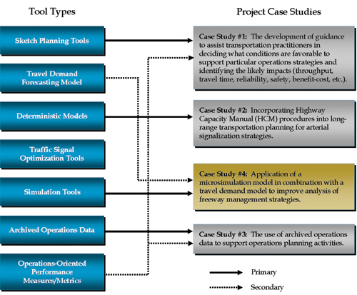 Figure 1 - flow chart - The figure shows that the four case studies represent a variety of the traffic analysis tool types. Each case study supports a primary tool type and several also support multiple case studies. Case study number four is highlighted to represent the contents of this document and it primarily supports the simulation tool type. It also includes travel demand forecasting model tools as a secondary tool type.
The main problem of interfacing travel demand models with microsimulation models is that the demands produced by demand models are not as capacity constrained as they need to be for use in microsimulation models. Demand models have a flexible capacity constraint; the traffic assigned to a facility during the analysis period can exceed its capacity by several orders of magnitude. Microsimulation models have a “storage space constrained capacity constraint”; the traffic assigned to a facility during the analysis period cannot exceed its capacity plus its ability to store the excess queues of vehicles. The result is that the microsimulation model produces unrealistic facility performance estimates when it is given unrealistic calibration year and future year demands.
The solution is to adjust the travel demand model demands to more realistic levels that reflect the physical limitations of the network (the flow capacity and the storage capacity). This section describes two case studies for applying simulation models in combination with travel demand models. The traditional approach described in the first case study performs these adjustments outside of the travel demand model. The second case study is an advanced approach that makes many of the demand adjustments within the demand model.
This case study documents the benefits as well as the pros and cons of integrating travel demand forecasting models with microsimulation tools for freeway operational studies.
Current travel demand models and planning analyses may underestimate the day-to-day benefits of operational improvements targeted at the reduction of vehicular traffic congestion. Underestimation of the ongoing benefits of relieving congestion results in a bias in the transportation planning and programming process in favor of capital improvements, which increase capacity over operational improvements.
Travel demand forecasting models are usually validated for regional characteristics. For example, the Contra Costa County Transportation Agency’s (CCTA) model, which was used for Case Study 4b in this document, includes a detailed zone system throughout Contra Costa County and the Alameda County portion of the Tri-Valley area. It was not designed for corridor analysis or sensitivity analysis of various freeway management strategies.
In general, travel demand forecasting models have the following limitations:
Because of these limitations of travel demand forecasting models, it is essential to apply microsimulation models for evaluating the full benefits of freeway management strategies.
This first case study involves a conventional application of a microsimulation model in combination with a travel demand model.
The travel demand model is used to estimate existing and future origin-destination (OD) demands for a freeway section. The calibration year OD was then adjusted to match the calibration year counts for the freeway. These calibration year OD adjustments were then carried forward to the future year forecasts and applied to the future year OD trip tables produced by the demand model. The microsimulation model is applied using the adjusted calibration year and future year OD tables.
The freeway performance is estimated exclusively using the microsimulation model. The demand model performance predictions are not used.
The goal of the Alameda County (California) Central Freeway Study was to prioritize a funding sequence among various combinations of all potential freeway improvement projects in the jurisdiction.
The Alameda County Central Freeway Study evaluated 10 miles of the I‑880 freeway from the Davis Street (SR 112) interchange to Whipple Road and five miles of I‑238/I‑580 freeway from 164th Street to East Castro Valley Boulevard. Figure 2 shows the freeway network in the study area. The Alameda County Congestion Management Agency's (ACCMA) official travel demand model (developed in Cube) was used to forecast future travel demand in the corridor, including ramp and mainline volumes on the freeways. Paramics microsimulation software was selected for producing measures of effectiveness (MOE) results of freeway operations for each alternative. Traffic conditions of morning and afternoon (AM and PM) peak hours were evaluated.
Surface streets were not modeled in the microsimulation model. Surface streets were included only in the ACCMA Cube travel demand model. Two freeway interchanges and 20 ramp junctions (on-ramps and off-ramps) were included in the microsimulation network.
The approach used is outlined below:
Figure 2. Alameda County Central Freeway Study Area
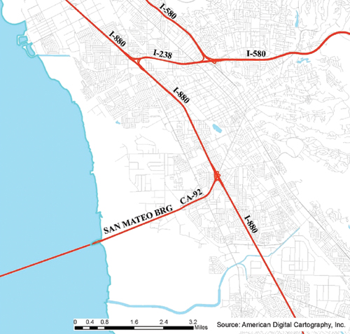 Figure 2 - map - The map shows the Alameda County side of the San Mateo Bridge in the San Francisco Bay area including the following routes colored in red to represent the facilities included in the model: I-880, I-238, I-580, and CA-92 (the San Mateo Bridge).
Figure 3 shows the flowchart of this traditional method. The details of these steps are explained in the following paragraphs:
The base-year travel demand model for this case study contained the land use data for 2005. The model’s loaded 2005 network (with traffic assignments) was used to generate the subarea network. The Cube software has a function to generate OD matrices (AM and PM peak-hour trip tables) based on a subarea network. Thus, analysts simply “cut” the large regional network into a smaller subset area and then run the scripts. For this case study, this process consolidated 3,000 zones (the regional model) into 43 zones of the subarea network.
Figure 3. Traditional Approach Flowchart
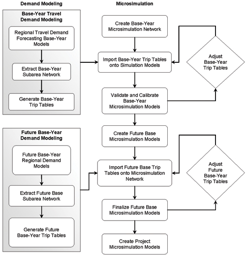 Figure 3 - flow chart - The flowchart shows the demand modeling and microsimulation processes for base-year and future base-year demand modeling for the traditional approach. This includes forecasting base and future year regional travel demand models, extracting the subarea networks, and generating the base and future year trip tables. The trip tables are imported into the microsimulation models. The base year models are then validated and calibrated. Future base and project microsimulation models are then created. The future base year trip tables are imported into the microsimulation model. Since the level of demand from the demand model usually cannot enter the network during the peak, the analysts needs to reduce the assigned demand by adjusting the base year OD matrices to remove unrealistic bottlenecks. These adjustments are then reimported in the microsimulation model and the future models are finalized. Lastly, project scenario networks are created based on the future base microsimulation networks.
Each microsimulation software package handles OD matrices differently. In Paramics, multiple OD matrices can be loaded onto the same network file. For example, one network file can contain two OD matrices: AM and PM peak hour. The zone numbers in Paramics network should be consistent with the subarea demand model’s zone numbers.
Once the base year OD matrix is imported into the microsimulation model, analysts start the validation and calibration processes.
In this study area, based on field data at certain locations on westbound freeway I‑580, the maximum capacity of the freeway was roughly 2,000 cars per lane. However, the demand model loaded the network with almost 2,500 cars per lane. During the initial microsimulation runs, the traffic flow of the westbound I‑580 was completely shutdown near the diverging point of the freeway I‑238, so the downstream freeway segments received very few traffic volumes. Since this level of demand cannot enter the network during the single peak hour, the analysts needed to reduce the assigned demand by adjusting the base year OD matrices to remove the unrealistic bottleneck. As a result, the downstream freeway segments received reasonable traffic volumes and the measure of effectiveness was able to be gathered and presented properly.
When the assigned traffic flow was reduced to something more realistic on freeway I‑580, some bottlenecks were found on both northbound and southbound directions of freeway I‑880. Analysts again checked the roadway geometry and adjusted the OD matrices in a second round. These trial-and-error processes require tremendous effort when the study area is relatively large. Calibrating and validating the microsimulation model for the base year according to the FHWA’s microsimulation guidelines (Federal Highway Administration, June 2004, Traffic Analysis Toolbox, Volume III: Guidelines for Applying, Traffic Microsimulation Modeling Software, Publication No. FHWA-HRT-04-040, – available at https://ops.fhwa.dot.gov/trafficanalysistools/index.htm) consumed a large portion of the budget.
The year 2025 future ACCMA models (with traffic assignments) were used to create future year trip tables. Analysts extracted the regional models into the smaller subarea. Cube scripts were applied to the subarea and generated the future trip tables.
The same percentages of volume adjustments (as were applied to the calibration year trip table) were applied to the future trip tables. In this case study, analysts used Microsoft Excel software to document all adjustments of the base-year trip tables. Thus, when future trip tables were created by the ACCMA model, analysts were able to simply copy and paste the adjustments (equations) to the future no-project and future project trip tables.
After the base year microsimulation model was complete, analysts copied the model and saved it as the future “no-project” network. New geometry was added on the network allowing for the incorporation or uploading of future year OD matrices in the models. Simulation runs were performed and the models were also checked. Therefore, project scenario networks were created based on the future base microsimulation networks. All estimates of measures of effectiveness for each project scenario were gathered and compared with the future “no-project” simulation models.
This case study demonstrated the benefit of combining a simulation model with a demand model to evaluate the benefits of a freeway improvement project.
The simulation model results showed that some systemwide benefits of certain project scenarios were off-set by the increased volumes. For example, one of the project scenarios was to modify the one-lane on-ramp to a two-lane on-ramp at the merging area from the I‑238 freeway to the southbound I‑880. In existing conditions, this capacity constraint (one-lane on-ramp) caused the queue on the westbound I‑238 and sometimes even spilled back onto the I‑580 freeway. When the ramp capacity increased from one-lane to two-lanes, it brought roughly one thousand more vehicles onto the southbound I‑880. These increased volumes resulted in more delay of the traffic flow on southbound I‑880. Thus, the overall travel time saving was less than the agency’s presumption.
At the end of this project, the benefits of applying microsimulation in combination with travel demand models were shown and helped the agency to prioritize the funding sequence of all project scenarios.
The traditional approach (adjusting the demand outside of the demand model) is feasible to perform manually (with the assistance of a spreadsheet) for small microsimulation study areas employing no more than 50 origin and destination zones. This approach becomes too laborious for larger study areas. Larger microsimulation study areas would require greater automation of the post-demand model adjustment process.
Besides the physical limits on the ability of the analyst to manually adjust large OD trip tables, there is also the theoretical concern that the demand adjustments are being made on an “ad-hoc” basis, without taking advantage of the behavioral models already incorporated at great expense in the demand model. The analyst simply reduces the calibration year demands produced by the demand model to match existing counts and then assumes that the same errors are also present in the future year forecasts produced by the demand model. This assumption does not take into account changes in the future network (more transit service for example) or the implications of reducing demand in one corridor on the operation of nearby corridors.
The goal of this more innovative approach to combining travel demand models with microsimulation is to reflect the effects of downstream weaving and queuing on upstream locations (the output of the microsimulation model) within the travel demand model itself. This procedure that includes validation of an estimated base year trip matrix in the travel demand model resulting in acceptable congested speeds and queues in the base-year simulation model as well as the development of a growth matrix, was used for the second case study described below.
The Tri-Valley area is nestled between major job centers in Silicon Valley and affordable housing supply areas east of the San Francisco Bay Area (San Joaquin Valley) in California. The cities in the Tri-Valley area (Dublin, Pleasanton, and Livermore) are also undergoing massive development in housing and employment. The primary transportation corridors serving travel to and through this area are already over-capacity today for several hours during the morning and afternoon peak periods. Significant volumes of traffic divert from the freeways to parallel local streets. The Alameda County Congestion Management Agency (ACCMA) initiated the Triangle Study to evaluate and develop a near term and long-range plan for sequencing improvements for practical traffic relief on the Tri-Valley freeways (I‑580, I‑680 and SR 84) in a cost effective manner consistent with the transportation needs in the area.
The regional travel demand model used for this case study was the Contra Costa Transportation Authority’s (CCTA) Decennial model. This regional model has 1,454 traffic analysis zones covering the entire Bay Area (Figure 4) with more detail in Contra Costa County and the Tri-Valley area. Full model runs were performed for the existing and future base years and a subarea highway network and associated trip tables were extracted (Figure 5).
Figure 4. Case II–Regional Model Highway Network
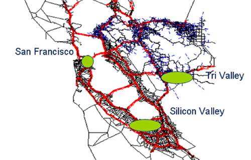 Figure 4 - map - The map shows the San Francisco regional highway network included in the model for this case study. San Francisco, Silicon Valley, and the Tri Valley are highlighted with green ovals to indicating greater detail for analysis.
Figure 5. Subarea Highway Network
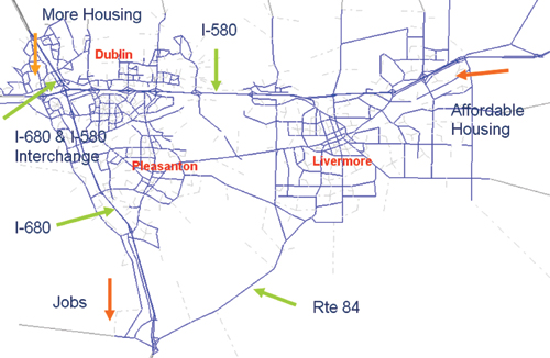 Figure 5 - map - The figure shows the subarea highway model network including the cities of Dublin, Pleasanton, and Livermore. Major routes including I-580, Route 84, and I-680 are indicated as blue lines, as well as the approximate locations of housing and jobs.
This example of an innovative approach of combining travel demand models with microsimulation models was performed as follows:
Of these steps, the most significant difference from a traditional approach is the implementation of a peak spreading algorithm and the iterative feedback between the travel demand model and the microsimulation model.
Key modeling procedures are described below.
The first step in the process was updating the regional model by adding network detail and splitting traffic analysis zones (TAZ) to allow for analyses of build out of the local city general plans and to reflect local access to the highway network. From the regional model, a subarea extraction process was used to create subarea networks and peak period trip tables. The full four-hour a.m. and four-hour p.m. traffic assignments were used to create the subarea networks to ensure that the full demand would be included. The subarea model had 600 traffic analysis zones.
Matrix estimation (ME) was used to create one-hour subarea trip tables from the four-hour subarea traffic assignments using known supply (capacity) and demand (counts and cut-through surveys) assumptions. The latest peak one-hour traffic counts were used to validate the base year demand model as well as review of cut-through traffic. In essence, the base-year peak trip matrix was factored to better replicate observed traffic counts, cut-through travel patterns, and most importantly regional capacity constraints. This procedure is outlined in Chapter Eight of the report, NCHRP Publication 255. Cube software and its companion program Analyst (matrix estimator) were used for this project.
Balanced traffic volumes between intersections are critical for running any matrix estimator relying on traffic counts as a seed into the process. If traffic volumes are not balanced on the freeway and arterial corridors, the process cannot reasonably find optimal solutions which balance. Ideally, counts should be balanced before the matrix estimator process is run. The volume balancing function in Synchro software is a useful tool to perform the volume checking. Figure 6 shows the locations of available traffic counts for the Triangle Study.
The subarea model was validated to establish criteria including comparisons of model data to VMT from the Caltrans Highway Performance Monitoring System (HPMS), total volumes and percent root mean square error (RMSE) by facility types and volume groups, traffic counts across screen lines, and the percentage of links falling within the FHWA validation curve. A list of the validation criteria used in this case study is provided in the appendix.
In addition to validating the travel demand model, the estimated demands were fed to the base-year simulation model to ensure that simulated congested speeds and queues were reasonable.
All members of the Technical Advisory Committee, including Caltrans and the participating local jurisdictional technical staff, were privy to the validation process.
Figure 6. Traffic Count Locations
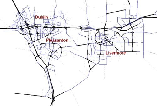 Figure 6 - map - The figure shows the subarea highway model network with traffic count locations highlighted in black within the cities of Dublin, Pleasanton, and Livermore. The locations cover almost all of I-580, and many major intersections within each city.
After the “fitted” at-capacity vehicle trip matrices were estimated for each time period (AM and PM peak periods), the increment of estimated growth between current and future conditions was calculated directly from the demand model and then added to the adjusted base year trip matrices. This process allows for the interplay of future growth while using a starting trip table which more appropriately represents existing at-capacity traffic patterns. The increments were added to the “unadjusted/original” forecasted models in appropriate time periods (AM and PM peaks) to produce adjusted model forecasts.
Adjusted Forecast Model = Future Base-year Forecast –
Original Base-year Model + Adjusted Base Model
The adjusted model forecasts were estimated in this manner for each alternative to ensure consistent comparisons of MOEs between project alternatives.
After the existing and future base-year travel demand model trip tables were validated, they were imported to microsimulation models which allow for the analysis of reduced capacity due to merging, weaving, and queuing. In this case study, CORSIM software was used to evaluate traffic operations on the individual vehicle level.
Vehicle queuing and throughput information (served vehicles) can be fed back to the travel demand model. For example, if the freeway congestion is caused by downstream merging/diverging traffic bottlenecks, the constraint of this freeway throughput is not correctly represented in travel demand models. Thus, the delay calculated by microsimulation models can be fed back to the travel demand model to have more precise analysis results.
In this case study, delay information from the microsimulation model (in the form of reduced capacity) was fed back to the demand model. Analysts reran the traffic assignment of the travel demand models to obtain a modified trip table matrix which reflects additional rerouting of traffic based on effects of queuing and bottlenecks. This “second round” modified matrix was used by the microsimulation models for validating and calibrating the microsimulation networks.
This feedback loop was applied only once in this case study since the resulting queuing and congested speeds in the simulation model appeared reasonable but, depending upon the number of alternative routes and level of congestion, could be applied iteratively. Users may refer to the ITS Benefits Assessment Framework Study for more information regarding appropriate linkages between models.
Figure 7 shows the flowchart of the innovative approach applied in this second case study.
Figure 7. Flowchart of Innovative Approaches
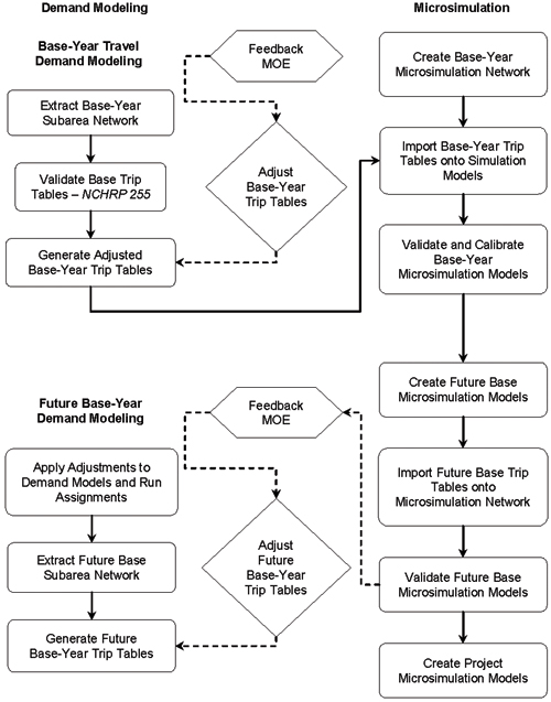 Figure 7 - flow chart - The flowchart shows the demand modeling and microsimulation processes for base-year and future base-year demand modeling for the second case study. The future base-year modeling process builds on the base-year modeling. This flow chart differs from the previous flowchart because it integrates feedback on the MOE.
The approach applied in this second case study takes into account known information about supply constraints (peak spreading) and travel demand patterns (cut-through traffic) as well as the effects of queuing and bottlenecks (microsimulation) on route diversion. This requires the iterative feedback between the travel demand model and the microsimulation model. While this “extra” step requires a level of effort, there is usually already a correspondence between the two models (since information must go from the travel demand model to the simulation model), which can be used to develop a correspondence in the “other” direction.
Also, as stated above in the discussion about Case Study 4a, if the trip tables that are fed to the microsimulation model do not take into account some level of peak hour spreading, the microsimulation models are difficult to calibrate and validate to existing conditions. This is particularly time-consuming and thus expensive for large-scale studies. Future levels of congestion simply exasperate the process. On the contrary, if analysts are not familiar with the appropriate application of a matrix estimation process in demand modeling, this procedure may take a significant amount of time. Many software packages provide this capability but, since there are many options in matrix estimating, engineering knowledge and judgment on what is happening in the study area are integral to making correct input adjustments and constraints such as setting confidence levels on origin-destination pairs, trip ends by traffic analysis zones, and the traffic counts.
While travel demand models reasonably forecast travel demand patterns which reflect a certain level of route diversion due to capacity constraints, they often fail when analysts assign trip tables representing high demands resulting in significant over-capacity conditions. By nature, a travel demand model (a macroscopic tool) will assign total volumes, regardless of whether the highway network supply can support it. Even though microsimulation models (a microscopic tool) will not allow the over assignment of travel demand (these vehicles are simply counted as “un-served”) this does not solve the problem when trying to output MOEs. In reality, the travel demand will “spread” to the shoulders and a certain amount of route diversion will occur. This is the goal of mesoscopic modeling.
Several software packages are developing the bridge between the macroscopic and microscopic (travel demand forecasting and microsimulation). Hopefully in the near future, analysts could have a more seamless integrated process between the two. In the mean time, some mesoscopic simulation tools can quantify impacts of upstream traffic congestion and measure queuing at intersections and merge points in a network. These tools integrate the feeding back of reductions in capacity information to the travel demand process. The innovative approach described herein attempts to apply this process without the availability of a reasonable mesoscopic tool.
The recommended approach to applying this process is to direct project resources (time and budget) to the validation of the future base scenario. The stakeholders will need to accept the results of the future base scenario so that the differences between alternatives can be used in the decision-making process. While validation of the models to base conditions is important, it is necessary to ensure that the sensitivity of the models to input growth assumptions is also validated. Then the model can be used to more reliably identify the differences in future alternatives.