Traffic Signal Timing Manual

Contact Information: Operations Feedback at OperationsFeedback@dot.gov

This publication is an archived publication and replaced with the Signal Timing Manual - Second Edition.

---

TABLE OF CONTENTS

• 7.0 DEVELOPING SIGNAL TIMING PLANS
• 7.1 OVERVIEW
  • 7.1.1 Signal Timing Process
  • 7.1.2 Frequency of Timing Updates
  • 7.1.3 Steps
• 7.2 Project Scoping
  • 7.2.1 Determine Objectives based on Signal Timing Policies
  • 7.2.2 Confirm Standards and Procedures
  • 7.2.3 Dividing the System into Sections
  • 7.2.4 Select Performance Measures
  • 7.2.5 Identify the Number of Timing Plans
• 7.3 Data Collection
  • 7.3.1 Traffic Volumes
  • 7.3.2 Intersection Geometry and Control
  • 7.3.3 Field Review
  • 7.3.4 Existing Signal Timing
  • 7.3.5 Intersection Analysis
• 7.4 Model Development
  • 7.4.1 Data Input
  • 7.4.2 Analysis
  • 7.4.3 Draft Timing Plans
  • 7.4.4 Final Timing Plans
• 7.5 Field Implementation and Fine Tuning
• 7.6 Evaluation of Timing
  • 7.6.1 Performance Measurement
  • 7.6.2 Policy Confirmation and Reporting
• 7.7 References

LIST OF FIGURES

• Figure 7-1 Project Scoping
• Figure 7-2 Traffic Volumes Summary Used to Determine Weekday Time of Day Plans
• Figure 7-3 Traffic Volumes Summary Used to Determine Weekend Time of Day Plans
• Figure 7-4 Signal Timing Process Once Project Scoping Is Complete
• Figure 7-5 Example intersection condition diagram
• Figure 7-6 Signal System Data Collection Sheet
• Figure 7-7 Use of a Signal Timing Model in Initial Assessment
• Figure 7-8 Cycle Length Selection
• Figure 7-9 Cycle Length Analysis – Volume-to-Capacity Ratio Summary
• Figure 7-10 Cycle Length Analysis – Performance Index, Delay, and Speed
• Figure 7-11 Key Elements to Consider During the Intersection Analysis
• Figure 7-12 Weekday Time-of-Day Schedule
• Figure 7-13 Saturday Time-of-Day Schedule
• Figure 7-14 Controller Markup
• Figure 7-15 Field Implementation Process
• Figure 7-16 Time Space Diagram (Before-and-After Study)
• Figure 7-17 Delay and Speed Summary (Before-and-After Study)

7.0 DEVELOPING SIGNAL TIMING PLANS

This chapter documents the process for developing signal timing plans. The intent of this chapter is to describe the steps necessary to develop a traffic signal timing plan for a series of intersections. These steps, along with calculations, must be made to produce a timing plan for field implementation. The information presented in this chapter builds on the concepts, guidelines, and information presented in the previous chapters.

7.1 OVERVIEW

Timing plans can be developed for an isolated intersection or several intersections on a coordinated arterial. At a single intersection an adjustment may be in response to a citizen complaint or agency staff member’s observation regarding a specific problem. Field observation by agency staff is often critical to identifying localized problems and solutions. This can include minor adjustments to the detector settings or fine tuning to adjust the split and/or offset at the problem intersection for the time of day during which the problem was observed. This may also include adjustments to pedestrian and clearance intervals in response to a perceived safety problem. These types of adjustments are essential for effective signal system operation. They are restricted to that particular intersection and do not usually consider the impact the timing changes may have on nearby intersections. These adjustments are solely driven by a localized change in traffic conditions (and in some cases geometric conditions) or the enhancement of existing timing at a single intersection. Care should always be taken to make sure the problem at a single intersection is not transferred to another location resulting in overall diminished system performance.

Area-wide timing is quite different in scope from localized adjustments. The area-wide timing is a systematic update to a group of coordinated intersections. It provides the appropriate and necessary timing plans for each intersection in terms of its individual needs as well as the combined needs of a series of intersections (1). This includes a system-wide cycle length that provides the best overall performance. There is a trade-off between the efficiency of the entire system and that of individual intersections, and good area-wide timing should strike a balance between the two. Equally important, the area-wide timing process considers the number of different timing plans required for varying levels of traffic demand and considers the best times and/or traffic conditions for the changes between plans. It includes a rigorous process of engineering and testing both in the office and the field to ensure that the timing plans being implemented are well suited for the conditions. Minor adjustments are an important aspect of traffic signal operations but are not a substitute for carefully updated area-wide timing.

7.1.1 Signal Timing Process

The signal timing process has eight distinct steps that can be tailored depending on whether the effort is a slight adjustment of the timing or is an area-wide or corridor retiming effort. The signal timing process steps were introduced in Chapter 2. Refer to Chapter 2 to ensure that the relevant policies and objectives are defined and incorporated in the scope of the project (the first step in the process). The steps include:

1. Project Scoping;
   • Review Policies, Determine Objectives, and Identify Problems;
   • Confirm Standards and Procedures;
   • Identify the study system, corridor, or intersections;
   • Divide the System into Sections;
   • Select Performance Measures;
   • Identify the Number of Timing Plans;
2. Data Collection;
3. Model Development;
   • Data Input;
   • Analysis;
   • Draft Timing Plans;
4. Field Implementation and Fine Tuning;
5. Evaluation of Timing;
   • Performance Measurement;
   • Policy Confirmation; and
   • Reporting.

The decisions and calculations made in these steps should be based on field data or first-hand observations of traffic operations at the subject intersection. This process is discussed in detail in Section 7.3 as it relates to developing timing plans for an area-wide project.

7.1.2 Frequency of Timing Updates

Traffic signal timing should be reviewed every three to five years and more often if there are significant changes in traffic volumes or roadways conditions. Retiming traffic signals every three to five years is generally considered to be good engineering practice. This frequency of signal retiming is particularly important for jurisdictions or localized areas within a jurisdiction in which land use changes lead to rapid changes in traffic patterns.

Key to the ability to identify the right frequency for signal timing updates is a proactive monitoring program. Monitoring should include information from sources external to the traffic signal operators, including planning or development review staff or other agency department staff that are in the field. It may also include citizen complaints collected from phone calls or through emails.

Signal timing should be revisited when any of the following occur:

• Increased demand or changing turning movements (5 to 10 percent; lower percentage change critical when intersections operate at or near capacity);
• Reduced traffic flow (typically 10 to 15 percent reduction);
• Changed vehicle mix (increased truck percentages);
• Construction activities on the study route or on a parallel route;
• Changed land uses associated with development or travel patterns due to shifts in employment centers;
• Observed queue spillback caused by oversaturation of adjacent traffic signal; or
• Other factors (such as the addition of a new traffic signal to a corridor associated with new development or changes in the roadway network).

These changes can be produced by a number of physical alterations to the roadway network, including new roadways, geometric changes to existing roadways, or added or relocated bus stops. Changes may also result from modifications to surrounding land uses, such as new or expanded residential, business, retail or educational facilities. Most communities experience many of these transformations over a period of three to five years. Changes in traffic flow and roadway network characteristics often lead to the need for new signal timing. Equally important, they may also require changes in the times of day during which the timing is implemented. In the case of reduced demand, they may also lead to situations in which signal removal or flash operation during certain periods of the day is appropriate.

These alternative approaches are typically used to determine when new timing plans should be developed:

• The agency may develop a regular schedule (e.g., three years) and retime 1/3 of their system annually.
• The agency may identify the need for qualitative new timing and selecting areas for retiming based on the observation of degraded performance or areas undergoing development or redevelopment. The latter is due to increased intersection delays or symptoms such as cycle failure (queues do not completely discharge during each signal cycle), spillback from left turn bays or between intersections, and unused green time on side streets.
• The agency may perform an engineering analysis of areas where signal timing may be warranted. This can be done through the use of a simulation or by methods that compare the performance of the existing timing system against its optimized timing performance developed with signal timing software (such as Synchro, TRANSYT 7F, TEAPAC or PASSER II).

In some cases, agencies have found that signal systems that initially require timing every three years may require less frequent timing (every five years) as neighborhoods and their attendant traffic flows mature and stabilize. However, the need for retiming should be reexamined every three to five years using a formalized process, such as described above.

7.1.3 Steps

This section describes a procedure to develop a signal timing plan for a series of coordinated intersections. The procedure comprises a series of steps that describe the decisions and calculations that need to be made to produce a timing plan that will yield an effective relationship between a series of signalized intersections. Each step is described in detail in the following sections. Figure 7-1 highlights the overall steps involved in a signal retiming project.

Figure 7-1 Project Scoping

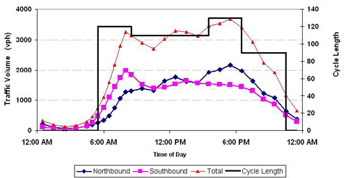
Figure 7-1 shows the flow of Project Scoping process beginning with Box - Scoping: Objective and Policy, Study Corridor or Network, Performance Measures, Number Timing Plans. An arrow points from to 2 Data Collection/Model Development/Final A curved labeled “Are Objectives Policy Met?” back 1. Another 3 – Field Implementation, Evaluation Refinement, Confirmation, Assessment/Reporting.

As highlighted in Figure 7-1, a key component of the signal retiming process is ensuring that the agency objectives and policies are being met with the signal timing plan development. Once these are confirmed, field implementation, evaluation and refinement, and reporting can be performed for the project.

7.2 PROJECT SCOPING

The project scoping is a key component of signal timing development. Project scoping establishes objectives, standards and procedures, study area, performance measures, and the number of timing plans.

7.2.1 Determine Objectives based on Signal Timing Policies

The signal timing policies and the associated objectives developed using the process described in Chapter 2 are the basis of the development of the area wide timing plan. Common objectives include reducing stops, delay, and travel time for a corridor. It is important in scoping a project to recognize that there is a point when the objectives of smooth traffic flow are irrelevant. Recent research conducted by the FHWA describes this in detail.

During the project scoping period, consideration should also be given to identifying known problems. The identification of these problems may be the result of public comments, staff observations, or known discrepancies with established policies. The identification of problems during project scoping may be an iterative exercise done in conjunction with determining objectives. In other words, previous problems may help shape the project objectives and/or, by clearly defining project objectives, deficiencies may be more apparent and easily addressed.

7.2.2 Confirm Standards and Procedures

Beyond the big picture policies determined above, there are also specific procedures and standards that should be confirmed as a part of the scoping process. The standards identify parameters used for the timing of change and clearance intervals, actuated timing settings, and pedestrian timing. The MUTCD defines several of these values and provides standard policies for agency use.

7.2.3 Dividing the System into Sections

The third step in project scoping is to identify logical groups (sections) of signals to be included in the timing process. The concept of sections is an important one. Typically, every intersection in a section changes to a new timing plan at the same time of day. Each intersection in a section likely operates in the same control mode—manual, time of day, or traffic responsive. For example, if an incident occurs and an operator would like to manually select an incident timing plan, the incident plan is implemented for every intersection in the affected section. In some cases during oversaturated conditions, intersections may be operated free to insure efficient green allocation.

Operational reasons are not the only justification for sectionalization. When traffic signal optimization software is used, the algorithm that is used to determine the best (optimized) timing is most sensitive to changes in smaller numbers of intersections than changes in an entire system equaling a large number of intersections (20 or more). Smaller groups of signals are easier to deal with. This includes management of data, collection of traffic data, implementation of new timing in the field, and fine-tuning adjustments to installed timing.

From the preceding discussion of sections, it should be clear that sections are autonomous groups of signals that can be controlled independent from other groups of signals. The groups of signals don’t have to operate the same cycle length; double cycling is evaluated when a common cycle length is not desirable. This understanding of sectionalization leads to the definition of the following section characteristics:

• The best size for a section is in the range of 2 to 30 intersections, understanding that as the number of intersections increase, the likelihood of a solution with a very small and/or discontinuous progression band also increases.
• It is possible for a single intersection to serve as a section, such as the case of an isolated intersection, or an intersection that is at the junction of two crossing arterials, each of which is a separate section.
• Section sizes can often exceed 30 intersections in cases where there are no logical breaks in intersection operation, such as in a large central business district where there is equal block spacing.
• If possible, section sizes should not exceed 100 intersections because the data management and installation requirements become unmanageable.
• Sections should include groups of intersections that are logical to control as a “unit.” This can be determined by common changes in traffic flow among all intersections (i.e., the peak period occurs at nearly the same time at all intersections in the section), by common changes in the time at which saturated conditions occur, by which intersections are impacted by the presence of incidents, or by the geographic location of the intersection.
• Adjacent intersections are considered when the distance between intersections is less than one mile and the traffic flow along the corridor is greater than 500 vehicles per hour per direction.
• To the greatest degree possible, sections should be created among groups of intersections whose operation does not have to be coordinated with intersections outside the section boundary. In this manner, one section can change its timing plan or control mode without concern for the impact on intersections outside the section. A commonly used natural boundary for a section is the intersection of an arterial with a freeway interchange.

However, there are also a number of misconceptions about sections, including:

• It is necessary for all intersections in the section to operate using the same cycle length—False. A common cycle length is not required. The definition indicates that all the intersections in the section must operate using the same timing plan, in which the cycle, split, and offset is defined for every intersection. However, the specific values do not need to be common to all the intersections in the section.
• It is not possible to coordinate sections with each other—False. Systems using common time bases for all intersections and operating on the same cycle length or a multiple of one another can be coordinated across all section boundaries.
• Intersections cannot be reassigned to different sections on a time-of-day basis—False. Some systems permit reassignment, which means it may be possible to vary intersection-to-section assignments by time-of-day.

As previously indicated, section boundaries are selected in a manner that will minimize the need for interaction with the signals in adjacent sections. For example, the signals on roadways connecting the two sections should be far enough apart that there is little need for signals in one section to be coordinated with the signals in the adjacent section. The traffic engineer should look for groups of signals that are surrounded by a buffer zone, which may be in the form of long intersection spacing, natural boundaries such as railroad tracks or bridges, changes in land use, or other factors that lead to differing traffic characteristics.

7.2.4 Select Performance Measures

As the project scope is defined, performance measures must be selected to evaluate the success of the retiming effort. Most operators use stops and delays as measures because they are the most sensitive to changes in signal timing and are the most obvious improvements that motorists will observe. However, several things should be considered prior to arriving at this decision’ including funding sources, the need to report results to the public, environment, etc. The FHWA and NTOC have projects that highlight a standard set of performance measures that emphasize the importance of travel time in addition to stops, delays, and average speeds.

During under-saturated conditions, stops and delay are the performance measures that are typically used. During oversaturated conditions, the objective is to minimize the time period during which these conditions exist and manage queue spillback between intersections. The performance measures in use include queue lengths, numbers of cycle failures, and the percent time that intersections are congested. This is accomplished by prioritizing movements and controlling the directions of queue build-up to avoid spillback and to minimize cycle failures.

Once the measures have been selected, the locations and routes that are candidates for performance measurement should be selected. Measurements should be made before new timing is installed and again at the completion of the signal timing process. In this way, the effectiveness of the retiming effort can be evaluated and communicated with agency management and the public. The before-and-after evaluation can also be used to identify locations where additional adjustments are needed because their performance falls short of expectations.

7.2.5 Identify the Number of Timing Plans

Since timing plans are developed for specific sets of traffic conditions, it is important to define the times of day when those traffic conditions exist, and therefore, the times of day when each plan should be used. It is also important to determine the number of unique sets of traffic conditions that will require signal timing plans. For example, tourist areas that experience a large fluctuation in traffic flow throughout the year may find it beneficial to develop timing plans for the tourist and non-tourist seasons of the year.

A number of factors constrain the amount of plans that can practicably be developed, including:

• Resources. Collecting data, developing plans, installing the plans and fine-tuning plans is a labor-intensive process; this work is constrained by available personnel and fiscal resources.
• Control Equipment. An important step in developing signal timing plans is making sure that the project engineer/technician has a full understanding of the controller type/equipment being used by the agency and its features, functions, and possible limitations of that equipment. Many systems have limits on the number of plans, phase sequences, and other signal timing operations that can be accommodated within the controller. This limitation should be carefully considered, and if resources are available for modernization they should be sought. If possible, a review of the equipment should be completed during the scoping process or, at a minimum, at the start of the project.
• Data Availability. Some plans, such as for snow storms, hurricanes, incidents, and store sales are based on conditions that occur on rare occasions. Collection of traffic data during these transitory conditions can be difficult if not impossible. Many agencies respond to these “unusual” circumstances through adjustment of existing plans. For example, agencies might increase the cycle length and slow down the speed of progression for plans that are used during snowstorms.

The process of selecting the number of timing plans and the times of day when they operate may be determined through a combination of reviewing traffic data along the corridor, such as 24-hour directional traffic counts, intersection turning movement counts (TMCs), and traffic engineering judgment. Ideally, the following steps are used to determine the number of different plans and appropriateness for time of day changes:

• For each section of the system (this is another reason why sectionalization is important), select a sample of representative intersections. These might be the most important intersections in the section (if some parts of the section are more important than others), or they may be a group of intersections whose traffic conditions are typical of those existing throughout the section. In either case, the set of representative intersections must include only locations that are adjacent to each other. Note that this process will require the availability of hourly counts for the entire time period being analyzed.
• Prepare a graph that plots the traffic volume as a function of time of day for the two or three most important intersections in the sample. Using the graph, identify the AM, PM and off-peak time periods for the sample. This step is executed using judgment in the same manner that a traffic engineer would manually determine the time periods for these conditions.
• Further analysis could include using the signal timing optimization model to determine whether the performance of the system would be improved with different timing plans. This requires substantially more data and may be completed later in the process. 7-7

Figure 7-2 has been prepared to represent the process described above. This figure shows the 15-minute periods that are included in each of the three major time periods (AM, PM and off-peak). The bounds or number of major periods can be varied as described above. Frequently, the greatest benefits can be found in breaking the off-peak period from the peak periods. For example, it may be desirable to add a noontime plan to accommodate increased traffic during the lunch hour. However, there must be a balance in the number of plans provided as many traffic signal controllers may need several cycles before achieving a coordinated offset and cycle following plan transition.

Figure 7-2 Traffic Volumes Summary Used to Determine Weekday Time of Day Plans

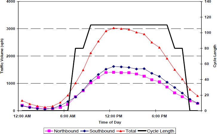
In addition to time-of-day plans, separate plans for weekdays, weekends or even specific days (such as Friday in a high weekend travel area) may be warranted based on variation in travel patterns and volumes. Figure 7-3 illustrates this process for a weekend time-of-day volume profile. For weekend time-of-day plans, it is common to use one timing plan for most of the day due to the balanced traffic volumes. A second timing plan might be used between uncoordinated operations and the peak traffic volumes.

Figure 7-3 Traffic Volumes Summary Used to Determine Weekend Time of Day Plans

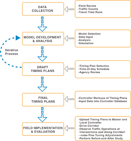
Through the above-mentioned process, the number of timing plans should be determined and included in the scope of work for the project. Figure 7-4 outlines the next steps used to develop signal timing plans that can be implemented in the field.

Figure 7-4 Signal Timing Process Once Project Scoping Is Complete

7.3 DATA COLLECTION

The data collection effort for a signal timing project can be quite costly and time intensive. This section summarizes several types of data used, as well as techniques that can be used to reduce the data collection effort and expense.

The data typically can be categorized as: traffic characteristics, traffic control devices, intersection geometry, and crash history. Data associated with each category are described in subsequent sections. The description focuses on the collection of data at an existing intersection. If the intersection does not exist, then estimates will need to be provided. In many instances, the data described herein will have already been collected as part of the engineering study associated with the signal warrant analysis.

7.3.1 Traffic Volumes

24-Hour Weekly Volume Profiles

Weekly traffic volumes should be collected at critical locations along the corridor. These locations are determined by the peak hour time periods and traffic patterns of the corridor. The weekly traffic volume profiles are an important element in the data collection effort and are used to identify:

• The number of timing plans used during the weekdays and weekend;
• When to transition from one timing plan to the next;
• Volume adjustment factors for developing turning movement counts; and
• Directional distribution of traffic along the corridor.

Weekly traffic volumes can be collected using tubes, system detectors, or other ITS devices that are in place along the corridor. Using system detectors or other ITS devices will reduce the time and cost of the data collection effort.

Turning Movement Counts

Turning movement counts are typically collected at each of the subject intersections under consideration for retiming. Depending on the traffic volumes and traffic patterns along the corridor, turning movement counts often only need to be conducted during peak periods, commonly the weekday morning, midday, and evening peak time periods. The daily traffic volume profiles should be used to identify the specific time periods for conducting the counts, as well as for use in developing volume adjustment factors for the weekend and/or off-peak traffic volumes. At some locations, the traffic volumes may be higher or more critical during the weekend time periods, which could lead to performing turning movement counts for the weekend and the weekday time periods. Additionally, seasonal traffic patterns may need to be considered and incorporated in the scope of work. Procedures for conducting, recording, and summarizing traffic counts are described in the Manual of Transportation Engineering Studies (2).

Intersection turning movement counts are collected for representative traffic periods. The traffic count should include a count of all vehicular traffic at the intersection, as categorized by intersection approach (i.e., northbound, southbound, etc.) and movement (i.e., left-turn, through, or right-turn movement), pedestrians, and vehicle type (including transit). If heavy vehicles are significant, the vehicular count should be further categorized by vehicle classification. The presence of special users at the intersection (e.g., elderly pedestrians, school children, bicycles, emergency vehicles, etc.) should also be documented.

Vehicular Speed

Data on vehicular traffic speed should be gathered to identify the approach speeds to the intersection. This is especially important in determining the signal phasing. In cases where the traffic signal is a new installation, detection layouts (number of detectors and location) are based on the approach speed. Traffic speeds are especially important when considering the detector timing described in Chapter 5.

Travel Time Runs

Travel time runs can be used to calibrate the existing analysis model and to compare the corridor operations before and after the new timings are implemented. Travel time runs are collected by driving the subject corridor and recording the delay, stops, and running time using electronic equipment. The following information can be collected from the study and later analyzed and used to develop the timing plans: average travel times, intersection delays, intersection stops, and speeds. Travel time and speed are common measures to report to elected officials and the public when doing signal timing improvements. It is also a good practice to monitor travel time as a means of determining the quality of existing timing and the need to retime.

7.3.2 Intersection Geometry and Control

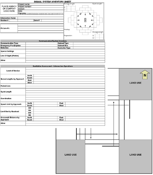
A site survey should be conducted to record relevant geometric and traffic control data. These data include: number of lanes, lane width, lane assignment (i.e., exclusive left turn, through only, shared through and right turn, etc.), presence of turn bays, length of turn bays, length of pedestrian crosswalks, and intersection width for all approach legs. An effective method for recording this information is with a condition diagram. An example condition diagram is shown in Figure 7-5.

Figure 7-5 Example intersection condition diagram

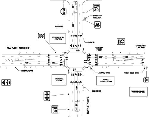
Figure 7-5 is an example intersection diagram containing a layout of the geometry including, number lanes, lane-widths, access points, and curb geometry. It also indicates locations signage, major attractions, parking, detectors other structures that may impact traffic movement.

Other information that can have an impact on signal operations include: approach grades, sight line restrictions, 85th percentile approach speed (if different from the speed limit), presence of on-street parking, presence of loading zones, presence of transit stops, dips in approach profile near the intersection, and intersection skew angle. Many of these factors will have an impact on the capacity of one or more movements at the intersection; they may also influence intersection safety.

If the intersection is being re-designed and existing conditions are the basis for documenting the benefits associated with the proposed design, then information about the existing detection design is also needed. This information includes: the number and location of existing detectors, their length and type, the number of detector channels associated with the detection for each traffic movement, and the type of controller memory associated with each detector channel and the detection mode.

All traffic control devices at the intersection should be inventoried during the site survey. This inventory should be categorized by intersection approach and include the speed limit signs, parking prohibition signs, turn movement prohibition signs, and one-way street signs. This information includes: the number and location of existing vehicular and pedestrian signal heads, phase sequence, use of overlaps, and signal timing settings.

7.3.3 Field Review

An important component of the signal timing development process is performing a field review at the signalized intersections and of the subject corridor. The key elements to consider are location and operation of signal equipment, intersection geometry, signal phasing, intersection operations, vehicle queuing, adjacent traffic generators, posted speed and/or free flow speed. The free flow speed will assist with calibrating the traffic model and establishing offsets that reflect the traffic conditions. However, the use of the free flow speed or posted speed should be discussed during the scoping process.. The field review is an excellent opportunity for the engineer or technician to become familiar with the operations, geometry, and potential constraints at the intersection, as well as to identify signal equipment (i.e., pedestrian indicators, detectors, or controller) that might not be operating properly. It is also an excellent opportunity to observe operational issues that would not be obvious by the hard data alone, such as queue spillback and approaches that are not serving the full demand. The data collection sheet shown in Figure 7-6 provides some of the information that might be useful during the field review.

One of the challenges of field data collection is to visit the corridor in a way that allows observation of the most critical time periods and important intersections. Identifying congested locations will be important to isolate where traffic analysis may need additional attention.

During the field review, if observations are made that reveal the signal timings are working adequately, then this should be noted. Many locations have traffic patterns that may be stable and have not undergone any geometric or signal phasing improvements, resulting in the existing operations being acceptable. This initial review may result in a smaller scope of project and could lead to focusing the effort on other deficiencies.

Figure 7-6 Signal System Data Collection Sheet

Turning movement counts are typically one of the more costly items in the scope of a traffic signal retiming study. FHWA published “Signal Timing on a Shoestring,” which provides some guidance on ways to minimize the data collection effort through a short count method or by estimating turning movement counts using link traffic volume data. These guidelines may be useful on corridors or networks where the traffic conditions are predictable. However, in developing areas where traffic patterns are rapidly changing, it may be more appropriate to collect two- to three-hour turning movement counts for the various study-time periods.

Use of existing detection for collection of turning movement counts is a practice recommended by the Institute of Transportation Engineers in a recent Informational Report.

7.3.4 Existing Signal Timing

This information is important to obtain at the subject intersections as it is used to develop an existing analysis model. Key information from the existing signal timing includes phase sequence, yellow and all-red intervals, pedestrian walk and flashing don’t walk intervals, minimum green, and detector settings. Additionally, if the intersection is operating in coordination, then the cycle length, splits and/or force-offs, offsets, and reference phases should be obtained from the existing signal timing. Some unique settings may be used in the field that can be identified by reviewing the existing signal timing, such as conditional use, overlap, or limitations in the phase sequence that can be incorporated in the existing model and timing development. The existing signal timing helps the user understand what currently exists in the field and provides a baseline for improvement.

7.3.5 Intersection Analysis

The building blocks of traffic signal timing rely on the analysis procedures highlighted in Chapter 3 and the intersection design elements described previously in Chapter 4. Combining the analysis with the design elements leads to the development of potential changes as a part of the signal timing process.

Assess Signal Phasing

During this step, data collected is used to determine a reasonable signal phasing for the conditions. Specifically, the key determinations in this step are whether a left-turn, right-turn, or pedestrian phase is needed for the various approaches in combination with the opposing approach. Guidelines for making these determinations are provided in Section 4.3. The phase sequence for leading or lagging left turns is described in Section 4.4. Pedestrian phasing is covered in Section 4.5.

Identify Traffic Signal Control Mode of Operation

During this step, the need for coordination should be evaluated. Additionally, whether the intersection should operate as pre-timed, semi-actuated, or fully actuated and whether it should be coordinated with adjacent signals is determined. It is important to consider the daily volume variation, prevailing approach speed, and objectives for the operation of the traffic signal. Guidelines for making this determination are provided in Section 5.2. If the intersection is part of a coordinated signal system, then the control mode is likely to be coordinated-actuated, where the minor movements are actuated and the major-road through movements are coordinated.

Verify Detection Design

An intersection's detection design depends on the mode of operation and the prevailing speed on each intersection approach. An intersection operating with pre-timed control does not require detection. In contrast, an intersection operating with semi-actuated or fully-actuated control will need detection for each actuated traffic movement. Guidelines for designing various types of detection are given in Chapter 4.

Refine (or Develop) Basic Signal Timing Parameters

During this step, the basic signal timing parameters are evaluated to determine the settings that will operate as a part of the timing plan. In the absence of coordination, these parameters control the green allocation and cycle length of the intersection. Intersections operated as part of a coordinated system will rely on the parameters to provide boundaries for the traffic signal timing and modifiers to the coordinated plans. It is very important that the basic signal timing parameters, as outlined in Chapter 5, be considered during any retiming effort as they may have a significant impact on both coordinated and uncoordinated operations. An evaluation of the basic timing parameters may be most effectively performed through field observation (e.g., performance of vehicle detection due to passage time settings or adequacy of clearance times).

7.4 MODEL DEVELOPMENT

This section addresses the steps needed to develop an analytical model for the signal retiming study. The first step is to select the model. Chapter 6 discusses the various models used for signal retiming and the use of manual methods.

Many computer-based tools are available to calculate and evaluate signal timing. Since many of these tools assume the presence of under-saturated conditions, it is important to recognize their capabilities and limitations. It is recommended that users develop a thorough understanding of the selected computer programs, their use, and how they relate to the field conditions.

The process of evaluating existing timing plans and developing new timing plans is iterative and involves detailed reviews of the information to successfully meet the objectives of the study. Several elements should be considered in the study:

• Establish a “standards and conventions” document (i.e., file naming, map settings, base data parameters, analysis settings) that provides the user with consistency through the retiming process;
• Review the plan development in levels or stages to ensure efficiency;
• Coordinate with the respective agencies; and
• Include quality assurance and quality control measures.

Figure 7-7 Use of a Signal Timing Model in Initial Assessment

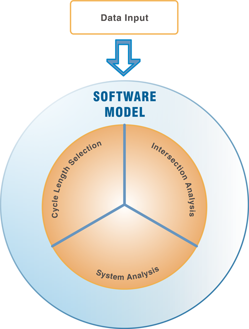
As shown in the figure, the data (traffic volumes, link network, lane geometry, existing signal timing, etc.) is coded in the software model and used to perform a cycle length analysis. From this analysis, a preferred cycle length is selected for the section based on the objectives of the study. This cycle length is refined through an iterative process of evaluating individual intersection operations with the system operations. Through this process, a final timing plan is developed and used during field implementation.

The requirements for developing timings for saturated and under-saturated conditions should be considered as the model is developed. Saturated conditions require careful distribution of green time that should include timing settings that seek to balance queue buildup and meter incoming demand. Because under-saturated flow tends to be stable (similar from one cycle to the next) traffic signal timing software can be used to calculate the best signal timing. Congestion exists if traffic conditions in the section are unstable with growing queues, spillback, cycle failure, or left turn bay overflows. Under these conditions, a separate process of calculating timing for saturated conditions should be used. In saturated conditions, congestion is difficult to avoid. Therefore, the control policy should be aimed at postponing the onset and/or the severity of secondary congestion, which is caused by the blockage of upstream intersections.

Turning movement counts may not capture the actual demand at intersections when conditions are oversaturated. Typical data collection measures for turning movement counts result in the traffic flow through the intersection rather than the actual demand that may still be part of a queue. It is important to validate the model to identify periods and locations where demand exceeds capacity.

7.4.1 Data Input

Depending on the size of the network, the data input work effort varies in intensity. With a few intersections the work effort is quick. However, if you have a corridor with 15 intersections or a downtown network with 100 intersections, the work effort becomes time consuming. To be successful, data input must be organized. The typical data used in the model include lane geometry, link speeds and distances, phase numbering, left- and right-turn phasing, existing signal timing (i.e., yellow and all-red intervals, pedestrian walk and flashing don’t walk intervals, minimum green, and detector settings), controller type, and coordinated reference phases. The data can be categorized into two sets: Network Parameters and Signal Timing Parameters.

• Network Parameters - These are parameters that are typically fixed through the analysis process. Examples of these include lane geometry, link speeds and distances, phase numbering, and left- and right-turn phasing. The link distances can be identified using aerial photography or a GIS map as base mapping in the software.
• Signal Timing Parameters – These are isolated signal timing parameters that are typically reviewed and modified during a retiming study. Examples of these parameters include yellow and all-red intervals, pedestrian walk and flashing don’t walk intervals, minimum green, and detector settings. These parameters are reviewed, and changes may be recommended at the beginning of the project. Once these parameters are reviewed and approved, they are used in the network and to develop the new coordinated signal timing plans. Chapter 5 describes methods to calculate signal timing parameters.

The network parameters and signal timing parameters are inputted in the selected model (i.e., Synchro, PASSER, TRANSYT-7F, or TEAPAC) to establish the base network. Certain parameters, such as traffic volumes and signal timing, may be inputted in the model through an automated process using the Uniform Traffic Data Format (UTDF). A base network is established for each of the study time periods (i.e., morning, midday, p.m., etc.)

Field observations should be compared with the traffic operation results for each time period in the model. If necessary, the base networks for each of the time periods should be calibrated using travel time, delay, and queue data collected from the field. Parameters within the models that can be adjusted to calibrate the existing base networks with actual field conditions include saturation flow rates, right-turning-vehicles-on-reds, lane utilization, and other parameters. A review of the calibrated model should be performed prior to moving forward with the timing plan development analysis.

7.4.2 Analysis

Several steps are typically used to analyze the different time periods when trying to establish a set of timing plans for the corridor. Figure 7-8 illustrates the process used to analyze the data and move towards plan selection.

Figure 7-8 Cycle Length Selection

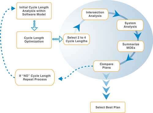
As shown in the Figure, the base network for each time period is used to select a cycle length, evaluate intersection and system operations, and identify the best plan based on the objectives of the study. These tasks are described below. Figure 7-8 illustrates the process used to analyze data and move towards plan selection for a specified time period. This cyclic includes developing initial cycle lengths, optimizing lengths through intersection analysis, system analysis their associated measures of effectiveness, comparing alternatives, ultimately selecting best frame. is discussed in detail paragraphs that follow.

Cycle Length Selection

Cycle length selection should reflect local policies and users of the system. Theoretically, shorter cycle lengths result in lower delays to all potential users. However, as tradeoffs are made among the various users, cycle length selection becomes more complex. As we consider more users, the cycle length may increase; each intersection is assessed for its cycle length requirement independently to determine a minimum cycle length.

The cycle length for the subject time period is determined based on the performance measures that have been identified for the system. The analysis of cycle length is performed using either simulation or signal timing software, during which the performance of the section is evaluated for a range of different cycle lengths. The range of cycle lengths used begins with the minimum cycle length (which is determined using Webster’s equation or a similar process) up to a maximum value determined by signal timing policy and controller capabilities. Typically, the range is evaluated at two second intervals.

After the initial analysis, two to four cycle lengths should be identified based on the objectives of the study and results of the initial analysis. The selected cycle lengths should be carried forward and analyzed for both intersection and system operations.

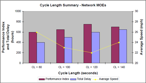
It may be helpful to summarize some of the MOEs from the different cycle length analyses to assist in selecting cycle lengths for further evaluation. As mentioned in previous chapters, a MOE that is often used to identify acceptable operations is volume-to-capacity ratio. A volume-to-capacity ratio of 0.90 or less is typically an acceptable measure; a volume-to-capacity ratio of greater than 1.0 would be a measure of oversaturated conditions (provided the assumed saturation flow rate is accurate). Figure 7-9 and Figure 7-10 illustrate intersection and system MOEs for various cycle lengths.

Figure 7-9 Cycle Length Analysis – Volume-to-Capacity Ratio Summary

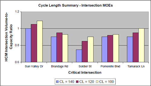
Figure 7-10 Cycle Length Analysis – Performance Index, Delay, and Speed

Once a cycle length is selected, the volume-to-capacity ratios, movement splits, minimum splits, and vehicle queues should be evaluated at each of the subject intersections for the two to four cycle lengths identified for further refinement. This analysis allows the user to assess if the cycle length will meet specific objectives of the study. For instance, if an objective is to ensure that pedestrian timings are accommodated within each phase split, then this assessment would make sure that the phase splits accommodate the pedestrian timings. The key elements are further shown in Figure 7-11. Figure 7-11 Is a list of key elements that should be considered during an intersection analysis. This includes the review movement volume-to-capacity ratios, splits, minimum and vehicle queues.

Figure 7-11 Key Elements to Consider During the Intersection Analysis

• Review movement volume-to-capacity ratios.
  V/C should be less than 0.90 (if possible)
• Review movements splits.
  Splits should accommodate traffic demand
• Review minimum splits.
  Are pedestrian times met?
  Is there an agency policy for violating pedestrian minimums?
• Review vehicle queues.
  Are the queues excessive?

Signal retiming is an iterative process that requires time to arrive at the most appropriate solution for the subject corridor. At the conclusion of the intersection analysis, the user should be able to identify one or two timing plans that would work for intersection operations.

Corridor Refinement - System Analysis

After the analysis is complete, a system analysis of the subject corridor or network should be completed to provide an analysis of:

• Vehicle progression along the corridor (i.e., Is there an acceptable bandwidth?);
• Intersection-to-intersection interaction (i.e., Do vehicle queues spillback?); and
• Left-turn operations (i.e., Is there benefit to lagging a left-turn movement?).

The user should use the following steps to ensure a detailed analysis is performed on the subject corridor or network:

• Review time-space diagram and/or traffic flow profile.
• Identify locations where the through band is being cut off (refer back to the objectives of the study) or where the front of the platoon encounters a yellow indication or only a few seconds of remaining green.
• Identify locations where movements, such as platoons on the major street or left-turns from a minor street, are being stopped.
• Identify locations where excessive queuing occurs.
• Evaluate locations for lagging left-turns.
• Evaluate locations where an “early green” may impact progression either beneficially or negatively.

In this system analysis, several signal timing parameters might be changed to improve the traffic flow, reduce vehicle queues, and meet the objectives the study. Some of these parameter adjustments could include offset changes, an increase in phase splits, and/or changes to the phase sequence of left turns on the major or minor streets. Care should be taken that if lagging left turn phasing is used, the requirements of the MUTCD are met so as not to create a yellow trap condition.

After this review is complete, the information associated with the intersection and system analyses should be summarized for the different cycle lengths. The summary comparison should be referenced with the objectives of the study to ensure the proper selection of a cycle length and resulting timing plan.

Simulation

After the various timing plans are reviewed or the best timing plan is selected, it might be desirable to evaluate the plans through a simulation program. Depending on the budget of the study, complexity of the corridor, and the degree of congestion, a simulation tool can be used to provide a more detailed analysis of the timing plans. The simulation results can be used to determine the best timing plan for meeting the objectives of the study and to increase confidence that the timing plans will operate as designed. Simulation does not need to be used on every retiming study, but it may be useful for evaluating timing plans with over-saturated traffic conditions.

The simulation program can be used to review the signal timing by incorporating the new timing plans in the simulation program and entering the traffic conditions for which they were developed. The simulation is then used to compare the selected performance measures resulting from the new timing with the measures produced by the existing timing or other cycle lengths. In this way, the potential effectiveness of the new timing can be evaluated. The simulation outputs can be used to identify locations where manual adjustments to the timing are required due to the presence of unusually long queues or other symptoms of poor performance.

Additionally, simulation programs have animated graphical outputs that approximate aerial views of the simulated network. These animated outputs permit visual assessment of system performance, a capability that cannot be duplicated by any other form of output, including time-space diagrams. Care must be used when reviewing animation from simulation models, as these should be reflective of an average run which can be selected only after review of the results. The Traffic Analysis Toolbox (3) describes simulation as useful for these and other applications, such as:

• To evaluate signals incorporating actuated-coordinated operations. Signal optimization programs treat these controllers as if they were pre-timed and then make suitable adjustments to approximate the operation of actuated controllers. The simulation program (if coded correctly) may provide a more realistic assessment of the effectiveness of the actuated controller within the section being evaluated.
• To confirm the likelihood of presence of queue spillback between intersections;
• To evaluate special features such as transit priority;
• To evaluate system performance in the presence of saturated conditions because these conditions are not adequately considered by signal timing optimization programs;
• To evaluate the effectiveness of manual adjustments to signal timing;
• To evaluate fuel consumption and emissions or system travel time resulting from a given set of signal timing; and,
• To demonstrate the improvements to public officials as it paints a clearer picture than numbers alone.

7.4.3 Draft Timing Plans

After the cycle lengths are evaluated, the intersections and system analyzed, and the timing plans compared, a preferred timing plan should be selected and carried forward to final review. This preferred timing plan is often called a draft timing plan.

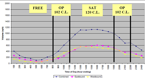
In addition to the draft timing plans, a time-of-day (TOD) schedule is developed that identifies the time periods for when the draft timing plans will be in operation. Figure 7-12 and Figure 7-13 illustrate a TOD schedule superimposed on a 24-hour traffic volume plot for a typical weekday and Saturday, respectively. On the weekday schedule, combined traffic peaks in the morning and evening during rushhour. On the Saturday schedule, traffic peaks in the middle of the day.

Figure 7-12 Weekday Time-of-Day Schedule

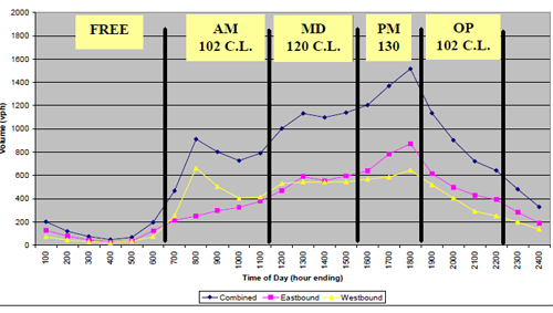
Figure 7-13 Saturday Time-of-Day Schedule

The TOD schedule will vary on corridors depending on the types of surrounding land uses. For instance, commercial corridors may have a low volume during the morning hours, begin to peak in the late morning, and continue to increase in demand through the evening time periods. Locations that consist of theme parks may have two peaks, one in the morning when users are arriving to the park and one in the late evening near the park closing. It is important to understand the surrounding land uses and how they impact the traffic operations throughout the day.

Typically, a summary of the MOEs and objectives of the study for each draft timing plan is prepared along with the draft TOD schedule and is submitted to the review agency. It is important for the parties to meet and discuss the draft timing plan to ensure that the objectives of the study are being met. After this review, the draft timing plans should be updated to reflect the final timing plans that will be used for field implementation.

7.4.4 Final Timing Plans

Once the review agency has completed its review and the comments have been incorporated into the draft timing plans, the timing plans are ready to be deemed final. A few steps need to be completed to prepare for field implementation:

• Identify the isolated and coordinated signal timing parameters at each intersection for each timing plan. Most software models provide a summary of this information by intersection. Typical parameters that might be modified as part of a retiming project are outlined below.
  • Coordinated Signal Timing Parameters
    • Cycle length
    • Splits or Force offs (depends on type of controller)
    • Offsets
    • Coordinated Phase
    • Phase Sequence (Leading or lagging left turns)
    • Vehicle Recalls
  • Basic Signal Timing Parameters
    • Minimum Green Time
    • Yellow and All-Red Intervals
    • Walk and Flashing Don’t Walk Intervals
  • Other Signal Parameters
    • Rest in Walk
    • Inhibit Max
    • Transition modes
• Identify the TOD schedule for the signal timing plans.
• Develop controller markups of the final timing plans and TOD schedule. Figure 7-14 illustrates an example markup for a controller.

Figure 7-14 Controller Markup

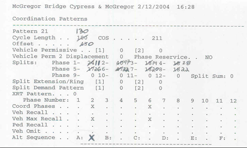
Once the draft controller markups are completed, a detailed review of this information should be performed to ensure that the correct timings have been marked up on the controller sheet. Additionally, this review may identify other existing timing parameters that are unique for a certain intersection that might need to be modified to ensure operation of the new timings. Depending on the agency, the final controller markups should be used to update the electronic files for each controller. Again, a detailed review of each electronic file should be performed within the agency or prior to sending the final files to the agency and being implemented into the controller. This process assists with minimizing the number of data entry errors during the process and allows for adequate preparation for field implementation. Finally, if yellow and/or red settings are being altered or if phasing is being revised, a formal approval by the agency’s traffic signal engineer may be required before the changes can be implemented.

7.5 FIELD IMPLEMENTATION AND FINE TUNING

Once the final timing plans have been completed and the controller markups have been prepared, the plans are ready to be implemented and observed in the field. Field implementation is the most critical part of the signal retiming process. Both science and finesse are needed to fully realize a good timing plan in the field. However, care should be taken to not draw an erroneous conclusion for a snapshot of time while on the corridor. Cycle-by-cycle variations occur, and one must be patient during observations. It is relatively difficult to see an offset error in the field when upstream intersections are releasing traffic early. Figure 7-15 illustrates the typical steps used during field implementation.

To assist with field implementation, a field notebook should be generated that includes hard-copies of the existing and proposed signal timing plans, time-space diagrams, traffic volumes, and a method for noting changes in the field.

Figure 7-15 Field Implementation Process

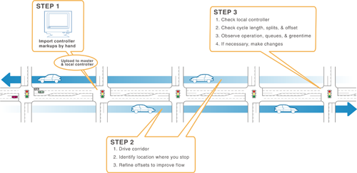
As highlighted in Figure 7-145, the final signal timing plans are uploaded from the traffic control center to the master controller (if applicable), where this information is transferred to each individual controller. Once this process has occurred, the engineers/technicians should drive the subject corridor or network to verify that the new timings are operational at each intersection. Observations of the intersection operations (i.e., Is the intersection operating the correct cycle length, phasing sequence, splits, etc.?) include side-street delay, major street left-turn delay, and review of vehicle queuing to ensure that the cycle length and movement green time are adequately dispersed for the traffic demand. If new signal timings are developed and implemented for the pedestrian Walk and Flashing Don’t Walk times, the engineer/technician performing the field implementation should check all of these times at each intersection to ensure that the crossing times are adequate and entered correctly in the controller database.

After visiting each intersection and confirming adequate operations, the team should drive the corridor to review vehicle progression and determine if any changes to the offsets or left-turn phase sequence is necessary. Depending on the history of the corridor and the number of proposed timing plans, field implementation and observations of the timings should consist of a minimum of three days (two days for weekday operations). If necessary, more days in the field should be added to ensure that the signal timings are operating acceptably.

Any changes that are made in the field should be documented in a field notebook and in the cabinet notebook at each intersection. These changes will be incorporated in the model network for developing as-builts of the implemented signal timing plans.

Once the signal timing is installed in a section, field observers or closed circuit television cameras should be positioned so that the entire system can be monitored. This activity will ensure that major problems, such as data entry errors, are quickly identified and corrected. Once the system appears to be operating correctly, it is necessary to identify the need for additional fine-tuning. This can be done through measurement of stops and delays at important intersections using the process of counting standing queues at intersections at regular intervals . As a final step, travel times should be evaluated using floating cars driven over the same routes that were followed during the evaluation of the “before” signal timing so that a comparison can be made.

If feasible, observing the traffic operations simultaneously both in the field and via a traffic management center can provide an efficient way to identify problem areas along the corridor due to short split times, excessive queuing, cycle failure, and/or hardware issues.

7.6 EVALUATION OF TIMING

With any type of project that is implemented in the field, the engineer should evaluate the performance of that project once it is in operation. Beyond the evaluation tools, a signal retiming project is no different. Some evaluation techniques include:

• Observing the traffic flow along the corridor and vehicle queues at individual intersections;
• Conducting “after” travel time and/or delay studies for the study network;
• Fielding phone calls and listening to the public;
• Verifying the new traffic operations are consistent with the agency policy and objectives of the study; and
• Comparing “before” and “after” measures of effectiveness from the analysis model and data collection.

A travel time and delay study is a common tool applied to most signal retiming projects. A disadvantage is that the travel time and delay information collected during the study is commonly limited to the through movements for the major route of the corridor and may not identify possible complaints from pedestrians or motorists crossing the arterial. Generally, if the objective of the study is to reduce stops and travel time along the corridor, a travel time and delay study is appropriate with observations of queue lengths on the side street approaches.

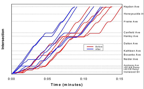
One of the summaries that can be generated from the study is a before-and-after projectile of vehicles along the corridor (i.e., a time-space diagram). The time-space diagram highlights the locations on the corridor that experience stops and long delays under the before and after conditions. Figure 7-16 illustrates a typical time-space diagram from a before-and-after study.

Figure 7-16 Time Space Diagram (Before-and-After Study)

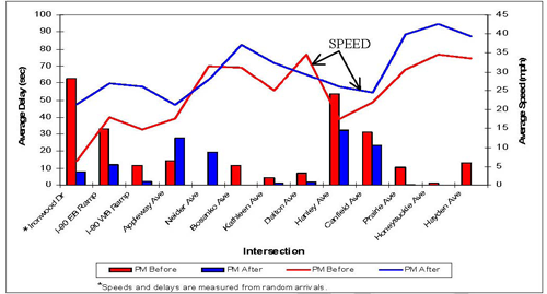
Another set of measures of effectiveness include delay and speed, which are typically used to evaluate the success of the project. Figure 7-17 illustrates a before-and-after summary of delay and speed for the corridor.

Figure 7-17 Delay and Speed Summary (Before-and-After Study)

7.6.1 Performance Measurement

It is critical to collect performance measures at an intersection to determine how well that intersection operates and serves the public. Reviewing and updating the intersection-specific timing and operational aspects of individual signalized intersections on a regular basis is extremely important, especially where changes in traffic volumes and/or adjacent land uses have occurred.

The most common performance measures used to describe signalized intersection operation are outlined in the Highway Capacity Manual (HCM). The methods used are vehicle oriented and focus on collecting manual data that is costly to gather. In most cases, it is not feasible for agencies to schedule manual data collection activities for unusual periods, such as evening school events or weekend peaks at shopping malls that do not allow timing plans to be developed to address all situations. Consequently, it is desirable to have signal systems collect their own data to assess performance through an integrated general purpose data collection module within the controller (4). However, obtaining meaningful real-time performance data from signalized intersections has historically been difficult because detection systems are not designed to provide good count information. Data is summarized in averages that may not be calibrated, and access to the information is limited to personnel managing the signal system.

7.6.2 Policy Confirmation and Reporting

After the data collection, signal timing analysis, field implementation, and evaluation are complete, there are two important final tasks that are needed: to confirm that the established policies were met and to prepare a final report.

The final report is an opportunity to confirm that the objectives of the retiming effort were met. Some agencies use this step in the process to inform elected leaders about the success of the project and to document future opportunities. A final report documenting the before-and-after study is typical and may be posted on the agency websites and/or passed along to news agencies for the public to view. However, more time spent developing a final report results in higher project costs and can reduce the time for the signal timing analysis, field implementation, and fine tuning efforts. During the scope of work process, it is important to determine the type of report necessary to assist with future retiming efforts, but this report should not take away time spent for the signal timing analysis and field implementation.

A report that is focused on the before-and-after study might include the following items:

• Introduction
• Travel Time and Delay Study Methodology and Analysis
• Travel Time and Delay Study Summary
• Savings Methodology and Analysis
• Savings Summary
• Summary

A report that is focused on the entire study might include the following items:

• Executive Summary
• Introduction
• Data Collection
• Signal Timing Development
• Timing Plan Summary
• Field Implementation
• Before and After Study
• Conclusions

The signal retiming process includes many steps to develop a successful set of signal timing plans. To promote a successful retiming project, it is critical to develop a comprehensive scope of work that is consistent with the agency objectives and local policy.

7.7 REFERENCES

• National Traffic Signal Report Card, National Transportation Operations Coalition, 2005.
• Manual of Transportation Engineering Studies, Institute of Transportation Engineers, 2000.
• Traffic Analysis Toolbox, Volume I: Traffic Analysis Tools Primer, Federal Highway Administration, June 2004.
• Smaglik, Edward, Sharma, A., Bullock, B. Sturdevant, J., and Duncan, G., “Event Based Data Collection for Generating Actuated Controller Performance Measures”, TRB Paper 07-1094, November 6, 2006.