Traffic Signal Timing Manual
Contact Information: Operations Feedback at OperationsFeedback@dot.gov
This publication is an archived publication and replaced with the Signal Timing Manual - Second Edition.
CHAPTER 6
COORDINATION
TABLE OF CONTENTS
- 6.0 COORDINATION
- 6.1 Terminology
- 6.2 Principles of Coordinated Operation
- 6.2.1 Coordination Objectives
- 6.2.2 When to Use Coordination
- 6.2.3 Fundamentals of Coordination
- 6.2.4 Summary
- 6.3 Coordination Mechanics
- 6.3.1 Cycle Length
- 6.3.2 Yield Point
- 6.3.3 Splits
- 6.3.4 Offsets
- 6.3.5 Other Coordination Settings
- 6.3.6 Pre-timed and Actuated Comparison
- 6.4 Time-Space Diagram
- 6.4.1 Basic Concepts (Time, Distance, Speed, and Delay)
- 6.4.2 Left-Turn Phasing
- 6.4.3 Bandwidth
- 6.5 Transition Logic
- 6.5.1 Example Application of Time Based Coordination Transition
- 6.5.2 Transition Modes
- 6.5.3 Operational Guidelines
- 6.6 Coordination Timing Plan Guidelines
- 6.6.1 Coordinated Phase Assignment
- 6.6.2 Cycle Length Selection
- 6.6.3 Split Distribution
- 6.6.4 Offset Optimization
- 6.7 Coordination Complexities
- 6.7.1 Hardware Limitations
- 6.7.2 Pedestrians
- 6.7.3 Phase Sequence
- 6.7.4 Early Return to Green
- 6.7.5 Heavy Side Street Volumes
- 6.7.6 Turn Bay Interactions
- 6.7.7 Critical Intersection Control
- 6.7.8 Oversaturated Conditions
- 6.8 REFERENCES
LIST OF TABLES
- Table 6-1 Harmonic cycle lengths based on street classification in Harris County, Texas
LIST OF FIGURES
- Figure 6-1 Time-Space Diagram of a Coordinated Timing Plan
- Figure 6-2 Phase and ring-and-barrier diagrams of intersection of two one-way streets
- Figure 6-3 Example of coordination logic within one ring
- Figure 6-4 Coordination using two rings
- Figure 6-5 Cycle Length and Split
- Figure 6-6 Fixed and Floating Force-offs
- Figure 6-7 Standard Offset Reference Points for Type 170, NEMA TS1, and NEMA TS2 Controllers
- Figure 6-8 Relationship between the Master Clock, Local Clock, and Offset
- Figure 6-9 Time-Space Diagram – Basic Concepts
- Figure 6-10 Time-Space Diagram – One-Way Street Operation
- Figure 6-11 Time-Space Diagram – Two-way Street Operation
- Figure 6-12 Sequence of Left Turn Phasing as Shown in a Time-Space Diagram
- Figure 6-13 Time-Space Diagram Example of Benefits of Lagging Left Turns
- Figure 6-14 Daily Cycle Length Fluctuations
- Figure 6-15 Transition Modes
- Figure 6-16 Cycle Length & Theoretical Capacity
- Figure 6-17 Alternating Offsets System of Intersections
- Figure 6-18 Quarter Cycle Offset Example Model
- Figure 6-19 Webster’s Optimum Cycle Length
- Figure 6-20 HCM Cycle Length Estimation
- Figure 6-21 How a phase times
- Figure 6-22 Non-coordinated phase operation with pedestrian timing completed before the force-off for that phase.
- Figure 6-23 Non-coordinated phase operation with pedestrian timing exceeding phase split
- Figure 6-24 Loss of coordination due to pedestrian call
- Figure 6-25 Vehicle trajectory diagrams showing the effect of changes in phase sequence
- Figure 6-26 Time-Space Diagram Example of Early Return to Green
6.0 COORDINATION
This chapter presents the concept of coordination of traffic signals. Coordination is a tool to provide the ability to synchronize multiple intersections to enhance the operation of one or more directional movements in a system. Examples include arterial streets, downtown networks, and closely spaced intersections such as diamond interchanges. This chapter identifies coordination concepts using examples from research and practice. It contains four sections. The first section provides an overview of coordination including a summary of objectives, the fundamental concepts, and expectations of coordination timing. The second section describes the concepts for coordination, its effect on time allocation, implementation issues, and time-space diagrams. The third section provides guidelines for developing coordination timing plans, and the fourth section describes complexities associated with coordinated operations. The intent of this chapter is to provide necessary background for the development of timing strategies.
6.1 TERMINOLOGY
This section identifies and describes basic terminology used within this chapter. Additional terms can be found in the Glossary section of the Manual.
Coordination
The ability to synchronize multiple intersections to enhance the operation of one or more directional movements in a system.
Double Cycle
A cycle length that allows phases to be serviced twice as often as the other intersections in the coordinated system. This is also referred as a “Half Cycle”.
Early Return to Green
A term used to describe the servicing of a coordinated phase in advance of its programmed begin time as a result of unused time from non-coordinated phases.
Force-off
A point within a cycle where a phase must end regardless of continued demand. These points in a coordinated cycle ensure that the coordinated phases are provided a minimum amount of green time.
Fixed Force-off
A force-off mode where force-off points cannot move. Under this mode, non-coordinated phases can use unused time of previous phases.
Floating Force-off
A force-off mode where force-off points can move depending on the demand of previous phases. Under this mode, non-coordinated phase times are limited to their defined split amount of time and all unused time is dedicated to the coordinated phase. Essentially, the split time is treated as a maximum amount for the non-coordinated phases.
Master Clock
The background timing mechanism within the controller logic to which each controller is .referenced during coordinated operations.
Offset
The time relationship between coordinated phases defined reference point and a defined master reference (master clock or sync pulse).
Offset Reference Point (Coordination Point)
The defined point that creates an association between the local clock at a given signalized intersection and the master clock.
Permissive Period
A period of time after the yield point where a call on a non-coordinated phase can be serviced without delaying the start of the coordinated phase.
Time-Space Diagram
A chart that plots the location of signalized intersections along the vertical axis and the signal timing along the horizontal axis. This is a visual tool that illustrates coordination relationships between intersections.
Yield Point
A point in a coordinated signal operation that defines where the controller decides to terminate the coordinated phase.
6.2 PRINCIPLES OF COORDINATED OPERATION
The decision to use coordination can be considered in a myriad of ways. There are numerous factors used to determine whether coordination would be beneficial. Establishing coordination is easiest to justify when the intersections are in close proximity and there is a large amount of traffic on the coordinated street. The MUTCD provides the guidance that traffic signals within 800 meters (0.5 miles) of each other along a corridor should be coordinated unless operating on different cycle lengths.
6.2.1 Coordination Objectives
Coordination is largely a strategic approach to synchronize signals together to meet specific objectives. While there are numerous objectives for the coordination of traffic signals, a common objective is stated succinctly in the National Report Card:
The intent of coordinating traffic signals is to provide smooth flow of traffic along streets and highways in order to reduce travel times, stops and delay(1).
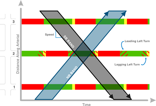
A well-timed, coordinated system permits continuous movement along an arterial or throughout a network of major streets with minimum stops and delays, which, reduces fuel consumption and improves air quality (2). Figure 6-1 illustrates the concept of moving vehicles through a system of traffic signals using a graphical representation known as a time-space diagram. The time-space diagram will be described in additional detail in later sections of this chapter.
The time-space diagram is a chart that plots ideal vehicle platoon trajectories through a series of signalized intersections. The locations of intersections are shown on the distance axis, and vehicles travel in both directions (in a two-way street). Signal timing sequence and splits for each signalized intersection are plotted along the time axis. It is very important these plots are to scale so that a consistency between units can be maintained. The time axis illustrates what motorists on the arterial will experience as they travel down the street. Left turns are shown as angled lines that either are operated with a concurrent green for the same direction or not.
Figure 6-1 Time-Space Diagram of a Coordinated Timing Plan
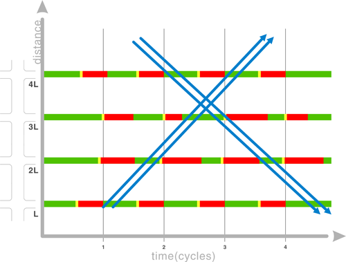
The result of signal coordination is illustrated on the time-space diagram above. The start and end of green time show the potential trajectories for vehicles on the street. It is these trajectories that determine the performance of the coordination plan. Performance measures include stops, vehicle delay, and arterial travel time; they can also include other measures such as changes in delay to transit vehicles or existence of spill back queuing between closely spaced intersections. In general, effective signal coordination should enable the engineer to meet the objective defined as a part of the study or relevant policies associated with the community. While the effectiveness of the coordination timing plan is directly related to the performance measures defined from the policy, it is also determined by the user experience and their perception of signal displays. Successful coordinated signal timing plans are usually characterized by both the audience and the measure:
- Downtown merchants may favor pedestrian traffic over vehicular traffic;
- A neighborhood may seek reduced traffic and lower speeds;
- The state may be interested in traffic volume throughput on state highways; and
- A transit agency may be concerned with signal delay to buses and/or light rail vehicles.
Ultimately, the perceived effectiveness of a coordination plan will depend upon local transportation policies, the elected leadership, relevant stakeholders, and the selected performance measures specific to the community.
6.2.2 When to Use Coordination
Numerous factors can be used to determine whether coordination would be beneficial. Establishing coordination is easiest to justify when the intersections are in close proximity to one another and when traffic volumes between the adjacent intersections are large. The need for coordination can be identified through observation of traffic flow arriving from upstream intersections. If arriving traffic includes platoons that have been formed by the release of vehicles from the upstream intersection, coordination should be implemented. If vehicle arrivals tend to be random and are unrelated to the upstream intersection operation, then coordination may provide little benefit to the system operation.
Information presented in the FHWA report, Signal Timing on a Shoestring, revealed that using both simple and complex procedures worked for identifying intersections for coordination. In short, when intersections are close together (i.e., within ¾ mile of each other) it is advantageous to coordinate them. At greater distances (i.e., ¾ mile or greater), the traffic volumes and potential for platoons should be reviewed to determine if coordination would be beneficial to the system operations. In both cases, the traffic conditions and the community policies should be considered as a part of the decision.
6.2.3 Fundamentals of Coordination
With the modern signal controller, coordination is accomplished by adding a layer of logic (that is, coordination logic compliments some basic features such as when a phase can begin or end) to the basic actuated logic used for isolated signal timing operations (discussed in Chapter 5). In previous chapters, the details of the controller settings were limited to those applied at isolated or independent intersections (maximum green, pedestrian timing, etc). Signal coordination establishes an additional set of time constraints among a series of signalized intersections by establishing a background cycle length (on each ring of the phase diagram). This cycle length includes a series of timers for each phase and requires the designation of one phase (in some cases one phase on each ring) as the coordination phase. This designation identifies the phase that will be the last (or first depending on your outlook) one to receive its allocation of green time. This coordinated phase is distinguished from other actuated phases because it always receives a minimum amount of assigned green time. While it is possible to have a portion of the coordinated phase be actuated, the important point is that there is a non-actuated interval for the designated coordinated phase(s) that is “guaranteed” every cycle for the purposes of coordination.
Figure 6-2 shows the intersection of two one-way streets, which results in a simple intersection with just two phases. It also shows the relationship between a phase diagram with movements assigned to the indications at the intersection, a ring-and-barrier diagram that illustrates the logic used in the controller for phase sequence and to establish the relationship between conflicting and complimentary movements, and the time-space diagram which would be used to display the relationship between this intersection and others along an arterial or within a street network (previously shown in Figure 6-1). This intersection only has one ring within the ring-and-barrier diagram and a simple time-space diagram. Phase 2 is identified as the coordinated phase. This intersection represents the most basic configuration for a signalized intersection.
Figure 6-2 Phase and ring-and-barrier diagrams of intersection of two one-way streets
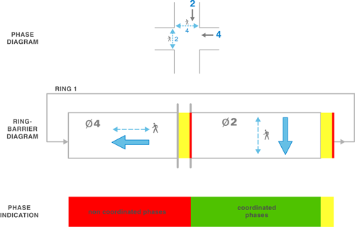
In an actuated-coordinated system, the first event in the cycle is the non-coordinated phase, which would serve the demand on that phase (in this case, just phase 4). If demand is less than the time allocated to that phase, it would gap out, and the remaining time for that movement would be reallocated to the coordinated phase (phase 2).
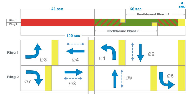
In Chapter 4, the ring-and-barrier diagram was introduced for a full-movement four-legged intersection, where Ring 1 consists of a sequence of phases and Ring 2 consists of the concurrent phases for the intersection, while the barrier separates intersecting movements (east-west and north-south). Figure 6-3 illustrates Ring 1 of the diagram and provides a graphical example of the phase indications for left-turn phasing. In this example, phase 2 is the coordinated movement, which means that phases 3, 4, and 1 all have an opportunity to use portions of their allotted time before phase 2 begins. If any time allotted for phases 3, 4, or 1 is unused, phase 2 will start before the normal start time (commonly referred to as early return to green) and then rest in green until its end point. The following sections of this chapter explain in more detail the nuances between different settings that affect the coordination relationship. Essentially, this is an additional layer of constraint (coordination logic) that can be applied to signalized intersections to improve the operation of a system of traffic signals.
Figure 6-3 Example of coordination logic within one ring
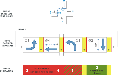
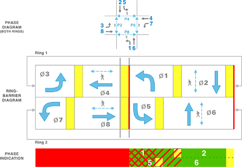
Figure 6-4 shows an example relationship between two rings (rings 1 and 2) at a typical 8-phase intersection. As seen in the figure, phase 5 uses less time than 1. As a result, phases 1 and 6 will time concurrently before phase 1 ends and phase 2 begins. In the time-space diagram, this concurrent operation of phases 1 and 6 is indicated by downward sloping left-to-right red bars, which indicate that the southbound movement is able to move through the intersection, but not the northbound movement. Additional examples of this are shown in section 6.2.4.
Figure 6-4 Coordination using two rings
The effects of coordination at an individual intersection depend on the timing plan and the operations of adjacent intersections. The coordination may be beneficial to a vehicle traveling between the two intersections, however it may negatively impact a pedestrian or vehicle crossing the street, waiting for the signal to provide the right of way. Many of the complaints from citizens related to the use of coordination address the restrictions placed that inhibits responsiveness to demand. The last section of this chapter describes the complexity of coordination in greater detail. This will be further exacerbated if the cycle length selected is unnecessarily long or the coordination plan is operating when traffic volumes are lower than typical (holidays that fall on a weekday).
6.2.4 Summary
Coordination applications can range from two signals controlling a diamond interchange, to dozens of signals controlling a combination of actuated and fixed time controllers controlling an arterial system that bisects a grid network. When applied, coordination strategies should follow the policies and resulting objectives for signal timing established by the agency. Once these are defined, performance measures can be established to determine whether the application is beneficial. Various performance measures can be used to evaluate signal coordination. Isolated intersection performance measures include delay, queue length, and safety; however, performance measures for coordinated systems may be slightly different. Evaluation methods include the number of stops reduced for the main street through movements or queue management.
Designating the traffic movement with the greatest peak hour demand as the coordinated phase is the most common practice. The coordination logic provides unused green time for the coordinated phase especially when demand for the other movements is low, which can result in fewer stops for the traffic movements with greatest demand. This is most typically through major street through movement.
As previously mentioned, other measures of effectiveness include reduced through movement and intersection delay, reduced travel times, lower emissions, lower fuel consumption, and maximized bandwidth. The Highway Capacity Manual quantifies some of these measures of effectiveness (through movement delay and resulting through-through travel speed), this manual does not. Instead, this chapter presents the concepts needed to operate a signal system. It should also be noted that from a system perspective the Highway Capacity Manual procedures are also not sensitive to the policy issues discussed here. The effectiveness of the signal system is (and should be) based on the policies and expectations for the various agencies. Measures of effectiveness can vary from travel speed, travel times, number of stops, pedestrian safety, pedestrian delay, transit efficiency, and overall intersection delay. In cases of public approval, the number of complaints or phone calls can be used as a measure of effectiveness, but may be biased toward a narrow perspective.
As previously described, well-defined objectives should be the starting point of the system evaluation. If an agency is focused on efficiency of automobiles, then the objectives will correspond to reduced travel time and delay for a given movement or intersection. The signal timing will reflect the priority given to the coordinated movement and, as a result, the through movement will have a higher percentage of the cycle time. However, if the agency wants to provide a system that is focused on moving people, then transit efficiency measures, such as percent on-time, ridership, and travel time, should be evaluated.
Many performance measures are difficult to quantify. Computer software programs can estimate many performance measures, including network delay, emissions, and fuel consumption, that are not easily measured in the field. However, one must be careful in selecting software tools, making sure they reflect the capabilities of the control software being used including timing settings and the detailed design of the detection system. Some performance measures are more difficult to quantify, which makes it more difficult to evaluate them objectively and to use them explicitly in an optimization exercise. These include public perceptions measured by phone calls (positive and negative), differences in perception of wasted time when conflicting traffic is present compared to when the intersection appears empty, and differences in perception of stops at minor intersections compared to major intersections. These measures require the traffic engineer to employ judgment—some might call it art—in balancing these less quantifiable measures with the other more scientific measures.
6.3 COORDINATION MECHANICS
Three fundamental parameters distinguish a coordinated signal system: cycle length, offset and split. These settings are necessary inputs for coordination. Figure 6-5 shows the cycle length and set of splits for an intersection, along with the offset between two intersections and the relationship to the master clock. There are several ways these inputs can be interpreted by the controller and thus a description of how the inputs are used to develop the relationship between the various intersections is provided here.
6.3.1 Cycle Length
Cycle length defines the time required for a complete sequence of indications. Cycle lengths must be the same for all intersections in the coordination plan to maintain a consistent time based relationship. (One exception would be an intersection that “double cycles,” serving the phases twice as often as the other intersections in the system.) The cycle length is measured from the deterministic point defined by the user. Coordination occurs most commonly along an arterial at an interchange or between at least two signals, but network coordination in downtown or other grid networks is also common. Professionals have determined cycle length through a variety of ways. The guidelines section of this chapter further discusses how to establish the cycle length for a coordinated timing plan.
6.3.2 Yield Point
The first component of coordination is often referred to as the yield point, but may be better defined as the deterministic point. This point is necessary for coordination to operate because it is a point where the controller makes a decision to terminate the coordinated phase. The controller will not leave the coordinated phase immediately because it has to confirm there is a conflicting call and time some coordinated phase clearance intervals (pedestrian clearance if resting in walk or just the yellow and red clearance).
Most controllers confirm what time-of-day plan should be running at this point in the cycle and transition to try to get to the appropriate plan at this point. It is also at this point that the controller will seek to serve the next phase in the sequence that has a call. In the instance where there is a call on any other phase, the coordinated phase would begin to terminate based on coordinated phase dwell state (walk or don’t walk) and clearance (yellow and red clearance time) and the next phase would receive a green indication based on the demand. If there is no demand on any other phase, the cycle would continue in the coordinated phase until the end of one or more yield periods, or the next occurrence of the yield point, where the controller would serve the phases in sequence. For each cycle, the controller decides at the yield point (or later with permissive periods) what phase(s) will serve.
6.3.3 Splits
Within a cycle, splits are the portion of time allocated to each phase at an intersection. These are calculated based on the intersection phasing and expected demand. Splits can be expressed either in percentages of the cycle or in seconds. Split percentages typically include the yellow and all-red associated with the phase; as a result, the green percentage is less than total split for a phase. For implementation in a signal controller, the sum of the phase splits must be equal to (or less than) the cycle length, if measured in seconds, or 100 percent, if measured as a percent (some traffic signal controllers are more finicky about this than others). In traditional coordination logic, the splits for the non-coordinated phases define the minimum amount of green for the coordinated phases.
Figure 6-5 Cycle Length and Split
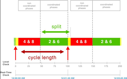
Figure 6-5 is a time-space diagram that shows a simplification of the signal indications for the coordinated and non-coordinated phases. The measured split for a phase consists of its green time, yellow change, and red clearance times. The cycle length is the sum of time for the complete sequence of indications. The measured split may be longer than what is input into the controller because of the early return to green. In an actuated-coordinated system, the cycle length must be measured from a defined observable point, typically the end of the coordinated phase green or beginning of coordinated phase yellow. Measuring the cycle length from the observed start of green at an actuated coordinated intersection will result in erroneous results because of the early return to green that can occur.
Force-offs
Force-offs are used in some controllers as an alternate way to control the phase splits. The force-offs are points where non-coordinated phases must end even if there is continued demand. The use of force-offs overlays a constraint on all non-coordinated phases to ensure that the coordinated phase will receive a minimum amount of time for each cycle.
In some controllers, this might be less than the pedestrian timing requirements, which offers the engineer some flexibility in timing. However, this flexibility comes at the price of potentially losing coordination if the controller does not return to the coordinated phase at its assigned time. Losing coordination under light traffic or only very occasionally due to pedestrian calls may be an acceptable option.
There are two options for programming force-offs in controllers, fixed or floating. The fixed force-off maintains the phase’s force-off point within the cycle. If a previous non-coordinated cycle ends its phase early, any following phase may use the extra time up to that phase’s force-off. This is beneficialif there are fluctuations in traffic demand and a phase needs more green time. One of the outcomes of this is that a phase later in the sequence (before the coordinated phase) may receive more than its split time (provided the maximum green is not reached). It should be noted that the phase directly after the coordinated phase will never have an opportunity to receive time from a preceding phase, regardless of the method of force-offs.
Floating force-offs are limited to the duration of the splits that were programmed into the controller. The force-off maintains the non-coordinated maximum times for each non-coordinated phase in isolation of one another. Floating force-offs are more restrictive for the non-coordinated phases. If a phase does not use all of the allocated time, then all extra time is always given to the coordinated phase. This is illustrated in Figure 6-6.
The maximum green timer, if allowed, may also result in the phase not reaching this force-off value. In addition to the maximum green timer, a definable controller parameter, known as Inhibit Max, may be invoked to prevent the controller from using the maximum green to limit the time provided to a phase during coordinated operation.
Figure 6-6 shows the difference between fixed and floating force-offs. The first row (“row a”) illustrates a scenario where demand exceeds the allotted green time and each phase is terminated at the respective force-off points. The second and third rows (“row b” and “row c”) illustrate the concepts of the floating and fixed force-off concepts. To better illustrate the differences in the two concepts, the demand for the phases are different. In this example, phases 1 and 3 experience a demand of 15 seconds (10 seconds shorter than the split time), and phase 4 experiences a demand of 40 seconds (15 seconds longer than the split time).
Figure 6-6 Fixed and Floating Force-offs
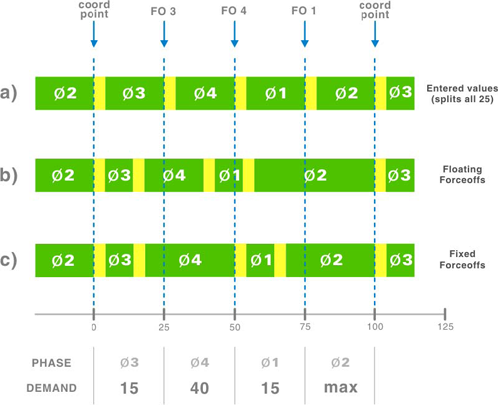
In this example phase 2 is the coordinated phase, phases 1 and 3 gap out, and phase 4 maxes out due to high demand. With fixed force-offs, the green time for phase 4 is extended to serve an increased demand up to the force-off point; in this case, it receives additional time from phase 3. The coordinated phase is given additional green time due to the previous phase (phase 1) gapping out. The green time is not taken from the other phases. For the same scenario under floating force-offs, phase 4 would be forced off even with the higher demand at its split value, 25 seconds. A Texas Transportation Institute report summarizes advantages and disadvantages of fixed force-offs (3):
- Fixed force-offs are useful to allow use of the time available from phases operating under capacity by phases having excess demand, which varies in a cyclic manner. This is the case when the phase(s) earlier in the phasing sequence is under capacity more often than the other phases.
- Fixed force-offs may reduce the early return to coordinated phases, which can be helpful in a network with closely spaced intersections. An early return to the coordinated phase at a signal can cause the platoon to start early and reach the downstream signal before the onset of the coordinated phase, which results in poor progression.
- Fixed force-offs reduce the early return to the coordinated phase which can also be a disadvantage. Under congested conditions on the arterial, an early return can result in the queue clearance for coordinated phases. Minimizing early return to coordinated 6-12
phases can cause significant disruption to coordinated operations. This disadvantage can be overcome by adjusting the splits and/or offsets at the intersection to minimize disruption.
Permissive Periods
A permissive period represents a period of time during the cycle in which calls on conflicting phases will be accepted. If a vehicle arrives after this period, it will have to wait until the next cycle to be served. In older actuated controllers, using coordinated operation, it was necessary to specify the permissive periods and force-offs for each phase. These values may be needed for entering signal timing plans in traffic controllers as well as traffic simulation models. Newer controllers generally automatically calculate (if allowed) the maximum permissive periods for the actuated phases. Care should be given to the selection of the coordination mode so as to not limit the benefit of larger permissive periods.
6.3.4 Offsets
The term offset defines the time relationship, expressed in either seconds or as a percent of the cycle length, between coordinated phases at subsequent traffic signals. The offset is dependent on the offset reference point, which is defined as that point within a cycle in which the local controller’s offset is measured relative to the master clock. It is not necessarily the same as the deterministic point (or yield point) within the cycle. The master clock is the background timing mechanism within the controller logic to which each controller is referenced during coordinated operations. This point in time (midnight in some controllers, user defined in others) is used to establish common reference points between every intersection. Each signalized intersection will therefore have an offset point referenced to the master clock and thus each will have a relative offset to each other. It is through this association that the coordinated phase is aligned between intersections to create a relationship for synchronized movements.
The location of the yield point and the offset reference point describes the relationship between the coordination plan at the individual intersection and the master clock.
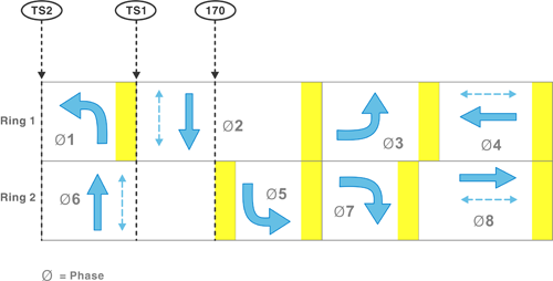
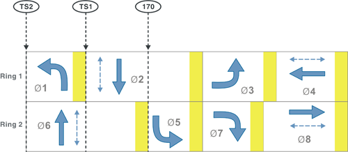
Different offset reference points are associated with each of the three major controller types: NEMA TS1, NEMA TS2, and the Type 170. The NEMA TS1 references the offset point at the start of the coordinated phases (e.g., phases 2 and 6). The NEMA TS2 references the offset point from the start of the green indication of the first coordinated phase (e.g., phases 2 or 6). The 170 typically references the offset point from the start of the coordinated phase yellow. For each of these controller types, software may allow variations of these designations. Figure 6-7 illustrates the differences of each offset reference point on a two-ring diagram.
Of the three reference points, only the use of the start of coordinated phase yellow is readily observable in the field. Under this type of designation, if Intersection B has an offset of 20 seconds after Intersection A, one should see Intersection B’s yellow twenty seconds after Intersection A’s yellow. For both NEMA designations, the use of start of coordinated phase green as an offset reference point is not a fixed point due to the variability in the start of green (early return to green) under typical actuated-coordinated operations. However, knowledge of the assigned split for the coordinated phase can allow one to calculate the observable fixed point in the cycle. In some cases, the start of coordinated phase Flashing Don’t Walk is used as an offset reference point. The majority of figures in this manual use the beginning of the coordinated phase yellow as the offset reference point, as it is easily observed in the field, although other references (including the HCM) often use start of coordinated phase green as the offset reference point.
Figure 6-7 Standard Offset Reference Points for Type 170, NEMA TS1, and NEMA TS2 Controllers
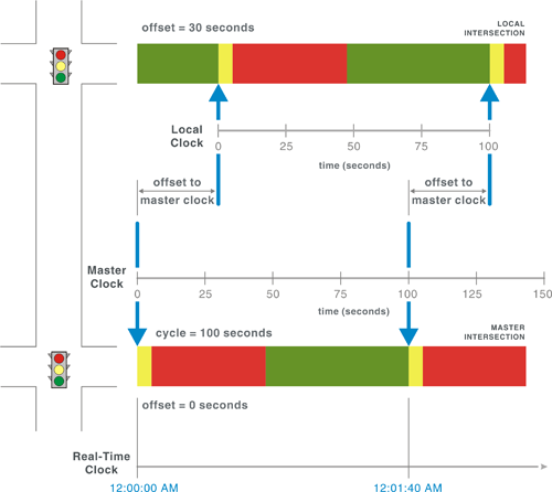
Once the reference point is identified, the offset is defined as the time that elapses between when this reference point occurs at the master clock and when it occurs at the subject intersection. Figure 6-8 illustrates this concept. In this example, the offset reference point is at the start of coordinated phase yellow, and a cycle length of 100 seconds is used for both intersections. The offset of the intersection on the bottom of the figure is zero and thus matches the master clock, which is referenced to midnight. The top intersection is set to an offset of 30 seconds. The coordinated phase begins its yellow at 30 seconds and 130 seconds (12:00:30 AM and 12:02:10 AM), always 30 seconds after the bottom intersection. The relative offset is observed by the user from intersection to intersection, but this can be different from the offset to the master clock.
Figure 6-8 Relationship between the Master Clock, Local Clock, and Offset
It is important that each intersection have consistent master clocks to enable time-of-day plans and preemption to use this as a base point. It is also important to understand that when the cycle length is changed, most controllers calculate a new “sync” point based on the master clock reference point. The start of the master clock, also known as Pattern Sync Reference, may occur at midnight or other times during the early morning, i.e. 1:00 AM or 3:00 AM. The selected time of day should avoid a transition during significant traffic volumes. This time-based reference requires the controller be configured to keep track of subtle issues, such as if the area follows daylight savings time and/or when daylight savings time begins and ends. For example, recent changes in Indiana in 2006 required all controllers in the state to be reconfigured to acknowledge daylight savings time. In 2007, every traffic controller in the country in states using daylight savings time had to be adjusted to account for a different start of daylight savings time.
6.3.5 Other Coordination Settings
There are a number of controller settings that may also be known as coordination modes in some controllers. Each controller type uses different coordination modes to give flexibility to the user. Such coordination modes include “Rest in Walk”, “One or more Permissive Periods”, and “Actuated-Coordinated Mode”. The modes operate in different manners, but each is designed to provide flexibility towards serving the users’ needs. Applications of these modes may vary with respect to high pedestrian volumes, transit priority, or leading and lagging left turns.
6.3.6 Pre-timed and Actuated Comparison
In pre-timed systems, typical of downtown closely spaced intersections, the time relationships are “fixed.” Today, most pre-timed systems use actuated controllers with phases recalled to their maximum time. In these types of systems, care should be given to the selection of walk times in order to provide a pedestrian friendly environment. Some controllers have a “fixed-time” mode which maximizes the walk time.
In systems with actuated phases, these relationships are less rigid and more complex. The “coordinator” uses many parameters to define where those time relationships vary and by how much. While the basic timing parameters of coordination are cycle length, splits, force-offs, coordinated phases, and offsets; it is very important to understand the complexities of these settings and their effect on coordinated actuated operation. The following section presents the theoretical construct of coordination in an attempt to break down the complexities into the basic fundamentals which are necessary to implement coordination consistent with the signal timing design undertaken.
6.4 TIME-SPACE DIAGRAM
The time-space diagram is a visual tool for engineers to analyze a coordination strategy and modify timing plans. The main components in a time-space diagram that are inputs include individual intersection locations, cycle length, splits, offset, left turn phasing (on the arterial in the direction of the diagram), and speed limit. The phase lengths may be approximations of their duration; in an actuated system this changes on a cycle-by-cycle basis. The outputs of a time-space diagram include bandwidth (or vehicle progression opportunities), estimates of vehicle delay, stops, queuing and queue spillback. The following sections describe the components of a time-space diagram and how the diagram can be used to evaluate signal coordination.
6.4.1 Basic Concepts
(Time, Distance, Speed, and Delay)
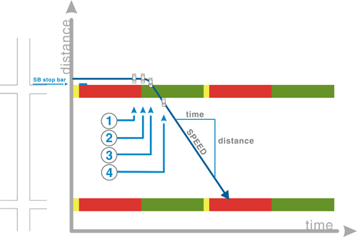
A time-space diagram is drawn with time on the horizontal axis and distance (from a reference point) on the vertical axis. The time is relative from the master clock described earlier. Vehicle trajectories are plotted on the time-space diagram and the difference in distance over time (distance divided by time, or change in y divided by x) represents the speed or a sloped line on the diagram. The trajectories always move left to right along with time, and as shown the distance traversed can be either northbound (bottom to top of the diagram) or southbound (top to bottom). Vehicles can have a positive or negative slope that indicates the movements on a street network. Stopped vehicles (no change in distance) are shown as horizontal lines. The assumed speed for coordination on the corridor may be the speed limit, the 85th-percentile speed, or a desired speed. The resulting speeds on the corridor are affected by the presence of other traffic, the signal timing settings, the acceleration and deceleration rates of the vehicles, and other elements within the streetscape. The acceleration rates are especially important considering the departures of standing queues at intersections.
Figure 6-9 shows the one-way street described in Figure 6-2 adjacent to another signalized intersection. In this diagram, the motorist experiences four different conditions in moving from a stop to the progression speed, these are:
- Vehicles delayed (no change in distance as time moves forward);
- Driver perception--reaction time at the onset of green;
- Vehicle acceleration; and
- Running speed of the vehicle (often assumed to be the speed limit or an estimated progression speed)
Figure 6-9 Time-Space Diagram – Basic Concepts
Vehicles on the time-space diagram are shown as trajectories between intersections. Vehicles that turn off of the arterial are considered separately from the through-through vehicles depending on the analysis. The vertical distance between two trajectories is the headway between vehicles.
Figure 6-10 shows more detail related to the range of possible trajectories for vehicles at the two intersection network described. The representation of the one-way street is continued for simplicity. The vehicle trajectories in this figure labeled 1 through 5 are described below:
- Vehicle travel (as in Figure 6-10);
- Vehicle from mid-block traveling through the downstream intersection;
- Vehicle from side street traveling to the downstream intersection, note the vehicle enters the arterial link during the red of the upstream intersection because it is on the side street turning left;
- Vehicle traveling at the progression speed through the intersections; and
- Vehicle delayed at the upstream intersection.
Figure 6-10 Time-Space Diagram – One-Way Street Operation
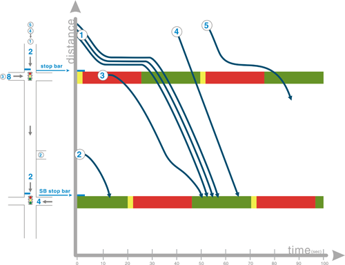
The time-space diagram illustrates the signal phasing for the coordinated phases for each of the signalized intersections. Each signal operates with two phases, with phase 2 as the coordinated phase.
Protected left-turn phases and two-way operation on the arterial street complicates the time-space diagram slightly. Figure 6-11 shows the additional phases and two-way operation on the arterial. A 100-second cycle length is assumed. Bandwidth is shown as the shaded area between the intersections.
Figure 6-11 Time-Space Diagram – Two-way Street Operation
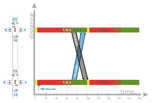
As illustrated in Figure 6-11, the left-turn phases result in less time for the arterial phase. Different types of phasing impacts the arterial street in various ways. Accommodating left-turning vehicles at signalized intersections is a balance between intersection safety, capacity, and signal delay.
Several traffic flow assumptions are used with time-space diagrams. As stated earlier, time-space diagrams typically consider the through movements on the street in deference to the turning traffic and other modes on the roadway. The time-space diagram and estimation of traffic flow are complicated by the interactions between pedestrians and turning traffic, vehicular interactions at midblock driveways, impedance from shared traffic lanes, and other users of the facility. Careful consideration of these conditions must be taken into account when using the time space diagram.
6.4.2 Left-Turn Phasing
As a phase times, the utilization of that green depends on the demand in close proximity or approaching the stop bar. In cases where traffic demand has not arrived, delaying the through movement may be beneficial. A corollary to this is that the traffic platoon from the upstream intersection may reach the downstream intersection too early. In either case, lagging the left turn may be beneficial to improve progression or make more efficient use of the green time.
The time-space diagram focuses on the arterial through movements (typically the coordinated phases). There are times when there are other concurrent movements occurring with the coordinated phase, such as the left turn movements. Within a time-space diagram, the left-turn movements are represented by hatching that is in the same direction as the coordinated phase. (In previous figures, phase 2 is a northbound movement and phase 6 is a southbound movement.)
There are situations when other movements are assigned to the coordinated phase, such as the left turn movements. This may be done within an interchange when a left-turn movement is particularly heavy or needs additional time.
Figure 6-12 Sequence of Left Turn Phasing as Shown in a Time-Space Diagram
As shown in Figure 6-12, the hatching for phase 5 is in the direction of phase 2 vehicle trajectories and the hatching for phase 1 is in the direction of phase 6 vehicle trajectories. When the left-turn movements occur at the same time (leading or lagging left turns), the hatching crisscrosses to show a period of time where through movements are not possible in either direction.
Lagging one or both of the left turns along an arterial to promote progression is common. Altering the order of the phases in the sequence may improve the use of the green provided, i.e. vehicles may arrive on green for their phase at the right time.
Lagging one of the left turns separates the start of the through phase from the start of the left-turn phase, which is particularly useful when upstream intersections from either direction are not equally spaced or have different offsets. This is demonstrated in Figure 6-13 below. Further discussion and examples are provided in Section 6.5.
Figure 6-13 Time-Space Diagram Example of Benefits of Lagging Left Turns
As shown in Figure 6-13, the bandwidth is increased (as compared to Figure 6-11) by lagging the left turns for subsequent intersections. The benefits of the lead-lag left-turn phasing are further enhanced with protected/permissive lead-lag phasing. By allowing vehicles to turn left during the permissive interval, required left-turn green phase time is reduced, which allows more green time for the coordinated movements. This technique is especially effective for coordinated arterial signals where the progressed platoons in each direction do not pass through the signal at exactly the same time. Al Grover recently completed a comprehensive evaluation of the impacts of protected/permissive phasing associated with coordinated signal timing in western San Bernardino County, California (4). Grover documented a 30- to 50-percent reduction in vehicle delay when comparing protected-only to protected/permissive left-turn phasing.
The Arizona Insurance information association studied lagging left-turn operation in 2002.Tucson, AZ, uses a lagging left-turn phase operation throughout the city. A particular benefit of lagging the left turn is that with PPLT control, the drivers have an opportunity to find a gap, but are providing an opportunity to clear the lane at the conclusion of the permitted phase. The Arizona Insurance information association studied this operation in 20025. The study found that Tucson, AZ had lower crash rates than the leading left-turn operations in the Phoenix, AZ. Area, and this benefit was attributed in part to the use of lagging-left phases. The City of Tucson uses lagging left-turn phase operation throughout the city.
Application of lagging left turns in conjunction with protected-permitted phasing presents the yellow trap to motorists. Understanding of yellow-trap issues is necessary before implementing lead-lag phasing (6). The “Yellow Trap” is a condition that leads the left-turning driver into the intersection when it is possibly unsafe to do so even though the signal displays are correct. During a signal indication change from permissive movements in both directions to a lagging protected movement in one direction, a yellow trap is presented to the left turning driver whose permissive left-turn phase is terminating. Use of the flashing yellow arrow as described in Chapter 4 alleviates the concerns associated with the traditional use of the protected-permitted in the doghouse display.
6.4.3 Bandwidth
Bandwidth is described as the amount of time available for vehicles to travel through a system at a determined progression speed. This is an outcome of the signal timing that is determined by the offsets between intersections and the allotted green time for the coordinated phase at each intersection. The bandwidth is calculated by the difference between the first and last vehicle trajectory that can travel at the progression speed without impedance. Bandwidth is a parameter that is commonly used to describe capacity or maximized vehicle throughput, but in reality it is only a measure of progression opportunities. Bandwidth is independent of traffic flows and travel paths and for that reason it may not necessarily be used by travelers. In other words, on an arterial with 10 signalized intersections, a bandwidth solution would be established to allow vehicles to travel through the entire system. In reality, one must consider how many vehicles desire to travel through all intersections without stopping.
A few important points to understand related to bandwidth:
- Bandwidth is different for each direction of travel on the arterial and dependent on the assumed speed on the time-space diagram:
- As additional intersections are added to the system, it is increasingly difficult to achieve and measure the impact of an additional signal:
- During periods of oversaturated conditions, bandwidth solutions may result in poor performance, often simultaneous offsets are more effective: and
- Timing plans that seek the greatest bandwidth increase network delay and fuel consumption.
6.5 TRANSITION LOGIC
Transition is the process of either entering into a coordinated timing plan or changing between two plans. Transition may also be necessary after an event such as preemption or loss of coordination due to a pedestrian crossing. In general, traffic signals do not operate within the same pattern parameters and cycle lengths at all times. The pattern may change during the day due to a number of reasons:
- Time-of-day scheduled changes
- Manual operator selection
- Traffic-responsive pattern selection
- Emergency vehicle, rail-road, or other preemption
- Adaptive control system pattern selection
- Corrections to controller clock
- Pedestrian demand
- Power loss and restoration
The time-of-day schedule determines what time a plan will be active. The simplest schedules typically define an a.m., off-peak, and p.m. peak for weekdays and a different set of plans for weekends. However, all controllers have extensive scheduling options that allow users to define several dozen plans that can be activated by individual day of week, month, pre-defined holidays, or major events.
When the controller clock reaches a point where it is necessary to change the coordination plan, the cycle, split, and offset are changed. If just the splits are changed, transition is trivial because the controller simply starts using the new splits. However, if either the offset or cycle change, the controller must shift the local offset reference point. This requires the use of an algorithm that may either shorten or lengthen the cycle to make that shift. That transition algorithm typically operates for one to five cycles, depending upon the transition mode selected and how much the cycle needs to be shifted. Consequently, the split durations during the period of transition may be different from either the previously defined splits or the new ones.
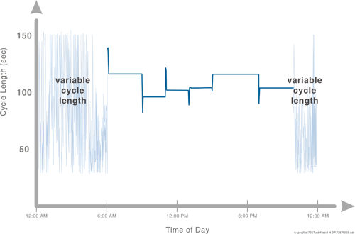
For example in the example cycle length plot shown in Figure 6-14, one can see the system runs with a fixed background cycle from 6:00 AM to 10:00 PM, with cycle changes at 9:00 AM, 11:00 AM, 1:00 PM, 3:00 PM, and 7:00 PM. During each of these plan changes, the controller goes into transition, resulting in variable cycle lengths for a couple of cycles to adjust to the new plan.
Figure 6-14 Daily Cycle Length Fluctuations
6.5.1 Example Application of Time Based Coordination Transition
Traffic signal coordination requires adjacent signals to operate at the same cycle length or at a multiple of the cycle length with pre-determined offset and coordination points. The most common method for achieving that specified offset is called time-base coordination, where coordinated signals are configured to use the same sync reference time, such as midnight or 3:00 a.m. When the signal is operating in a coordinated mode, it can calculate when the current cycle should begin by effectively counting forward from that sync reference time. The definition of the “start of cycle” depends on the offset reference point used by that signal, such as the start of green for a coordinated phase. The transition is initiated to re-align the local zero point (when the cycle begins) with the system sync reference time (when a timing plan is initiated).
As an example of time based coordination, consider a signal that is operating a coordination pattern that calls for a 90-second cycle and a 20-second offset, with 12:00 a.m. as the sync reference time. From this information, we know that this signal should begin a 90-second cycle at 20 seconds after 3:00 a.m. (3:00:20 a.m.) and every 90 seconds thereafter. An adjacent signal operating a pattern with the same cycle length but an offset of 45 seconds should begin a 90 second cycle at 45 seconds after 3:00 AM (3:00:45) and every 90 seconds thereafter. Hence these two signals will always have the same relative offset of 25 seconds (the difference between the two absolute offsets of 20 seconds and 45 seconds).
When a signal controller begins to operate a new coordination pattern, it must establish the cycle length and offset of that pattern. The same applies when re-establishing an offset after a cycle is disrupted by preemption or a pedestrian time that exceeds the split time. By calculating back to the sync reference time (12:00 a.m. in the above example), the controller can determine when the offset reference point is scheduled to occur within the current cycle. In general, the next start-of-cycle time will be several seconds earlier or a few seconds later than the current cycle start time. The larger the difference between the two cycles and/or the offset values of the two patterns, the longer the transition will take. While central or master-based systems typically communicate the selection of a new timing plan to all signals in a group at the same time, the actual transition logic is executed independently at each signal, without explicit regard for the state of adjacent signals. Most controllers allow three or four transition modes, which govern the precise details of how the signal resynchronizes to the new cycle and offset. The transition modes differ significantly from one controller manufacturer to the next. Some vendors may also refer to transition as offset seeking, offset correction, or coordination correction (7). The next section gives a brief overview of signal timing during transition for the most commonly available transition modes. However, no matter which mode is selected, traffic control can be significantly less efficient during the transition between timing plans than it was during coordination.
6.5.2 Transition Modes
There are three basic techniques for achieving an offset transition: dwell, lengthen, and shorten. The first technique is to stay (dwell) in the coordinated phase(s) until the new offset is achieved. That is, the current cycle is increased in length as needed, with all the additional time being assigned to “dwelling” or coordinated phases. The second technique also expands or adds to the cycle length as needed, but distributes that additional time between all phases. The third technique shortens the cycle length, taking time from all phases to the extent allowed by their minimum green settings and any pedestrian activity during the phase.
To avoid an excessive cycle length or phase greens that are too short during transitioning, it is common for controllers to limit the maximum amount of adjustment that can be made in one cycle. If such a limit is imposed, and it usually is, the signal may not be able to complete a given offset transition within one cycle. Signal controllers also commonly compute their adjustments so that transition is completed in a set number of cycles for the worst case scenario, typically a maximum of three to five cycles.
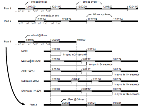
The most common transition modes in signal controllers in the United States include Dwell, Max Dwell, Add, Subtract, and Shortway, of which at least two or more modes are offered. (8) Figure 6-15 portrays two timing plans where the gray sections indicate when the coordinated phase is green and black sections indicate when the coordinated phase is red. Switching from Plan 1 to Plan 2 entails (for simplicity’s sake) no change to the cycle length, but a 24-second shift in the offset. Figure 6-15 also shows a separate timeline for each of five types of transition between Plan 1 and Plan 2. The descriptions of these modes discuss the example in Figure 6-15:
- Dwell – At the next display of green in the coordinated phase, the controller begins transition by holding (or dwelling) in this state until the new local zero point is achieved, at which time the signal is considered in sync and begins the new timing plan. As shown in Figure 6-15, this adjustment appears as one prolonged cycle. In general, this transition mode may result in an uneven allocation of split times during transition. It can be a very helpful mode to use when troubleshooting a coordinated system because it is very deterministic.
- Max Dwell – This modified version of Dwell also adjusts the start of the cycle by extending the green time of the coordinated phase. However, only a limited amount of extra green time may be added to each cycle. The example in Figure 6-15 is constrained to add no more than a certain percentage (20% is used in the example) to the cycle length, thus two cycles are required to achieve coordination.
- Add – This mode synchronizes by shifting the start of the cycle progressively later, by timing slightly longer than programmed cycle lengths. The Add mode increases the green time of all phases in the sequence, whereas the Dwell modes add time only to the coordinated phase(s). This is illustrated in Figure 6-15, where Max Dwell and Add both increase cycle lengths by a certain percentage (20% again is used), but the allocation of extra time to the coordinated phase is less in Add mode because extra green time is distributed proportionally amongst all phases. If a signal is subject to preemption, selecting the "Add-only" transition prevents splits on the phases omitted during preemption from being reduced during the transition period. The only real disadvantage of this mode is that if a cycle needs to shift one second backwards, it must shift the entire cycle forward one second less than the cycle length. This results in longer cycles during the transition period that could potentially cause unexpected storage problems in left turn lanes or between closely spaced intersections.
- Subtract – This mode shifts the start of the cycle progressively earlier, subtracting time from one or more phases in the sequence (subject to their minimum green time requirements). As shown in Figure 6-15, Subtract mode decreases all phases in the cycle by a certain percentage (20% is assumed) during transition. Though Subtract mode takes three cycles in Figure 6-15, the total transition time of three short cycles is equivalent to the time taken by two long cycles during Add transition.
- Shortway – This mode (also sometimes called Smooth) resynchronizes by applying either Add or Subtract transition logic, choosing the mode that presents the “shortest path” to achieving sync. The specific details of this mode, such as its name and the exact logic for determining the “shortest path”, can vary significantly from one controller vendor to the next. In general this is the default mode on most controllers and is typically appropriate to use, unless the signal is subject to preemption.
Figure 6-15 Transition Modes
6.5.3 Operational Guidelines
The example shows the effect transition has at a signal. Adjacent signals that change patterns simultaneously may take different amounts of time to complete their offset transitions, depending on which method is used and the size of the change required. In addition to disrupting the progression of vehicles between signals, offset transitioning artificially lengthens or shortens phases, leading to inefficient use of green time or unusual queuing. Therefore, it is best to avoid changing patterns during congested conditions when the signals need to operate at maximum efficiency. A peak-period pattern is best implemented early to ensure all offset transitioning is completed before the onset of peak traffic flows. Similarly, it is desirable to avoid frequent pattern changes.
When using the subtract transition technique, the new cycle length may be close to the sum of the minimum phase green times (or pedestrian times), meaning only a small adjustment in cycle length can be made by shortening. In this case, it may take many cycles to complete an offset transition. Hence, it is not practical to require the controller to use the subtract technique exclusively. To avoid this problem and allow use of the subtract technique when it works well, most controllers offer some version of the Shortway method. If the user selects this option, the controller will investigate both add and subtract techniques and automatically choose the one that will complete the offset transition (get the signal "in step" or "in sync") most quickly. Field experience and laboratory experiments have shown that Shortway typically provides the least-disruptive effects on traffic than any other methods, except in very rare cases. Many studies have also shown that excessive changes to timing plans, in an attempt to match traffic patterns closely and improve performance, can be a detriment because the system never achieves coordination for more than a few minutes at a time. Because of this, it is generally recommended to remain in a coordinated pattern for at least 30 minutes.
In locations with low pedestrian demand, it may be desirable to allow coordination to be lost when a pedestrian requests service. Care should be taken in using this mode of operation if vehicle progression performance is valued; a few pedestrians may cause one or more signals in a coordinated system to be in transition almost all of the time.
6.6 COORDINATION TIMING PLAN GUIDELINES
This section provides guidelines for selecting coordination settings. The information provided is based on established practices and techniques and some acknowledgement that additional research is necessary on this subject. The guidelines address the following topics:
- Coordinated Phase Assignment
- Cycle Length Selection
- Split Distribution
- Offset Optimization
Each of these topics is addressed separately in the remainder of this section.
6.6.1 Coordinated Phase Assignment
At each intersection, a coordinated phase is designated to maintain the relationship between intersections. Common practice is to designate the main street through phase as the coordinated phase because the coordination logic in most controllers dwells in this phase, and additional time provided to what is normally the busiest movement results in better performance. In many cases this is phases 2 and 6 for the main street through phases.
With some applications, assigning a phase other than the major street through movement has proven effective. A diamond interchange where queue management strategies are desirable is one example where a traffic signal may operate more effectively with such a designation.
6.6.2 Cycle Length Selection
Cycle length selection should reflect local objectives and users of the system. Theoretically, shorter cycle lengths result in lower delays to potential users. As we consider more users, the cycle length may increase and tradeoffs are made between competing objectives. Cycle length selection may be completed independently or by considering a system of intersections, but in most cases a first step is to assess each intersection for its minimum cycle length.
Each intersection is assessed for its cycle length requirement as a part of the selection process. The result is typically different “optimal” cycle lengths at the intersections. As these intersections are aggregated into systems, decisions have to be made regarding whether to include the intersection in a systems and which system to include the intersection in. There are cases where intersections are included in a coordination strategy which results in longer cycle lengths for the other intersections in the system. One should always consider whether intersections with long cycle length requirements would better operate independently of the system.
Cycle length selection is typically based on traffic data that is collected during representative periods. In reality, there is a wide variety of volumes that occur throughout the operation of the timing strategy. Automated data collection would improve the data and ultimately the cycle length selection, particularly at sites such as shopping districts that experience heavy weekend traffic that often is problematic for agencies to collect.
Similarly, because pedestrian timing may influence cycle length, various timing strategies are used to ensure effective coordination (8). The effect of pedestrians is further described in the next section. A key decision is whether pedestrians will be accommodated within the coordinated cycle length. In cases where pedestrian volumes (and the resulting actuations) are low, a pedestrian call may not be accommodated within the cycle length which will result in temporary disruption to the coordination timing.
The selection of a cycle length affects intersection capacity and delays. Longer cycle lengths can increase capacity, but only marginally. Shorter cycle lengths usually result in reduced delays. Thus, the objective of choosing a cycle length is to determine the smallest value of cycle length that provides the desired level of vehicular capacity at the intersection while being appropriate for the needs of other users such as pedestrians.
The selection of cycle length should also be influenced by the desired progression speed for a roadway. This is a complicated geometric relationship (to be discussed later) that must be recognized when selecting cycle length. Cycle lengths that are too long may increase congestion rather than reducing it due to the impacts of long waiting queues on side streets and the arterial alike. Cycle lengths also result in establishing relationships between the intersections and in some cases some values work better than others due to the time space relationship between the intersections.
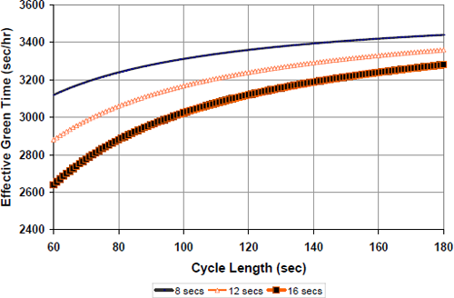
In general, it is preferred that the cycle lengths for conventional, four-legged intersections not exceed 120 seconds, although larger intersections may require longer cycle lengths(9). Theoretically, intersection capacity increases as the cycle length becomes longer because a smaller portion of the time is associated with lost time. However, it is important to recognize that the improvements are modest and this assumes that all lanes are operating with saturated flows. This requires that turn bays are long enough to provide sufficient demand to a particular movement; auxiliary lanes are more likely to be blocked with longer cycle lengths. As shown in the figure, the change of cycle length from two minutes (120 sec.) to three minutes (180 sec.) results in a modest 2 percent increase in capacity. This calculation was made by estimating the start-up delay resulting from the signal changes, as it relates to the number of times that the signal intervals change during the course of an hour. The message conveyed by the information presented in Figure 6-16 is that one should avoid placing too much emphasis on longer cycle lengths as a panacea for congested conditions.
Figure 6-16 Cycle Length & Theoretical Capacity
Manual Methods
A manual methodology for determining cycle lengths in a traffic signal network was first developed in Los Angeles. The City used a traffic signal timing strategy that was elegantly simple for its robust grid system. Most of the signals in the City had permitted left turns with signals at 1/4-mile spacing. A 60-second cycle length was selected and the green time was equally distributed to the cross street traffic and the arterial. Given these timings and spacing, a vehicle traveling at 30 miles per hour would reach the next 1/4-mile signal in 30 seconds, or half of a cycle length. The result is in an “alternating” system of offsets between subsequent intersections as shown in Figure 6-17. This system permitted two-way coordination along corridors. Under this configuration, the cycle length must be carefully selected with regards to the signal spacing and the anticipated or desired speed in the system. Although the optimization models used today can provide additional refinement to the coordination plans developed using this manual method, this method of alternating offsets serves as a reliable default timing strategy.
Figure 6-17 Alternating Offsets System of Intersections
Although the simulation and optimization models used today can refine the ways in which signals are timed, the alternating offset methods of yesteryear still work well as reliable default timing strategies10.
A similar method of manual coordination timing can be applied to downtown grid networks. This method has been deployed in downtown Portland, Oregon by separating intersections into a quarter cycle offset pattern. The block spacing in downtown Portland is fairly uniform and relatively short (280 feet) and the grid is a one-way network. Each subsequent intersection is offset by a quarter of the cycle length, which is selected to progress traffic in both directions. The result is a progression speed that is dependent upon the cycle length. This approach establishes a relationship in both directions of the grid and permits progression between each intersection in each direction based on the speed that is a result of the selected cycle length and the block spacing. As shown in Figure 6-18 cross-coordination throughout the grid is achieved using the quarter cycle offset method. This approach can be adjusted to account for turning movements within the grid and subtle modifications to the distribution of green time.
Figure 6-18 Quarter Cycle Offset Example Model
Some agencies have established fixed cycle lengths for various types of streets based on intersection spacing, signal phasing, travel speeds, and pedestrian crossing requirements. As an example, Harris County, Texas, uses cycle lengths shown in Table 6-1 below (11).
| Minor Arterial (seconds) | Major Arterial (seconds) |
|---|---|
| 60 | 90 |
| 70 | 105 |
| 80 | 120 |
| 90 | 135 |
This ensures a consistent approach is taken throughout the system for working between individual signals and intersecting corridors. This approach also suggests that the absolute value of the cycle length is less important than maintaining a relationship between adjacent systems of traffic signals.
Critical Intersection Methods (Webster, HCM)
Much of early research regarding cycle length selection recommended evaluating the intersections identifying the critical intersection which was typically the intersections with the highest demand. A cycle length is established for this location and is selected so that it will be sufficient to maintain undersaturated conditions. This fundamental assumption is currently being investigated to determine if there are further strategies for dealing with oversaturated conditions.
The critical intersection approach considers a signalized intersection in isolation to other intersections and for this reason may not always yield the optimum cycle length. Most of the analytical tools developed for cycle length selection focus on undersaturated flow (12). The tools also do not consider the constraints of the intersections beyond the lost time and saturation flow rate. These critical intersection approaches to cycle length selection are primarily for isolated intersections and are all based on the assumption that vehicular delay is most important. This approach analyzes the intersection with the heaviest traffic to determine a minimum cycle length and used that to set the remaining intersections. The first step is to consider each intersection as though it is isolated to determine the minimum (optimum) cycle length needed at each intersection, as though it were isolated(13). The traditional models use Webster’s model to determine optimal cycle length. Webster used computer simulation and field observation to develop a cycle-optimization equation intended to minimize delays when arrivals are random. (14) The formula is as follows:
Equation 6-1
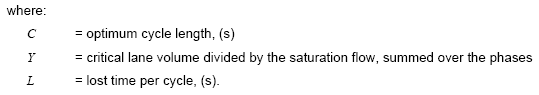
Figure 6-19 Webster's Optimum Cycle Length
In practice, much of the assessment of signalized intersections is completed using the Highway Capacity Manual (HCM) procedure on “Signalized Intersections.” The HCM provides few pieces of guidance on cycle lengths, but also notes limitations to the methodology. The current methodology does not take into account the potential impact of downstream congestion can have on intersection operation. Nor does the methodology detect or adjust for turn-pocket overflows and the impacts they have on through traffic and intersection operation.
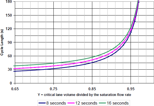
The HCM offers a quick estimation method for the selection of a cycle length. The formula for cycle length estimation is as follows:
Equation 6-2
![C = L / [ 1 - (min(CS,RS) / RS) ]](images/eq6_2.png)
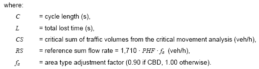
Primarily, this calculation is intended for planning-level analyses. This equation suggests that as the intersection approaches capacity, the cycle length should increase up to a maximum value, which the HCM suggests is set by the local jurisdiction (such as 150 seconds). The minimum cycle length suggested for use is 60 seconds. The equation does not explicitly address the pedestrian crossing requirements, left turn type and minimum green times necessary to meet driver expectancies.
Figure 6-20 HCM Cycle Length Estimation
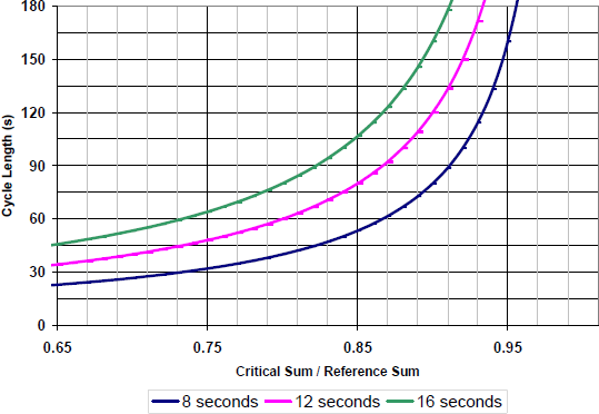
In both Webster’s and the HCM’s estimation, the sum of the critical lane flows is a representation f the demand at the intersection. The critical lane is defined as the intersection approach with the reatest demand of all the approaches that are serviced during a given signal phase. For example, during the main street phase, on a street with two-way traffic, the critical lane would be the one lane n either direction that has the greatest demand. Y is the sum of the critical lane flows divided by 900, which is the percent of available intersection capacity that is in demand. If Y = 1, the intersection is saturated and the equation is no longer applicable. The situations where longer cycle lengths degrade intersection performance are a result of specific elements that lead to poor performance.
Longer cycle lengths will increase congestion in cases such as when:
- Upstream throughput exceeds downstream link capacity. Long cycles may move more vehicles through an intersection than can be handled downstream
- Turning bay storage is exceeded. Long cycle lengths may cause vehicles in left-turn bays to back up into through lanes. In a similar manner, long cycles may cause through traffic to back up beyond turn bays, restricting their access
- Increased variability in actuated green times. Long cycles result in high variability in the side street green time used, which may result in poor arrival types at the downstream intersection. This is particularly noteworthy when split times exceed 50 seconds (15).
The delay experienced by a motorist depends on cycle length and volume. Higher volumes always lead to longer delays. Shorter cycle lengths reduce delay, provided they do not result in inadequate intersection capacity. Oversaturated conditions require special considerations, and these models are not valid during that range of conditions.
Network Approaches
The network approach to cycle length selection considers multiple intersections to determine an optimal cycle length. Most applications of network approaches use signal timing optimization models.
There are a number of computer programs that can be used to assist in selection of a cycle length. The Federal Highway Administration's (FHWA's) Traffic Analysis Toolbox describes additional resources (https://ops.fhwa.dot.gov/trafficanalysistools/toolbox.htm). Three of the more popular programs of this type are Synchro, PASSER™ II, and TRANSYT-7F (16).
These signal timing optimization models consider the network being analyzed and determine an optimal solution based on a given set of inputs. The range of cycle lengths is based on the users input. The optimization models use the individual intersection characteristics, the volume to capacity ratios of each intersection, the link speed, and the distance between the intersections to estimate the performance for each individual cycle length and resulting plan. The models make assumptions based on the inputs related to the splits and offsets to determine performance measures that can be compared to timing policies. Because the models are imperfect a significant amount of effort is necessary to take an initially screened plan to a point that can be field implemented. The timing policies described previously, the optimization policies, and the criteria for determining which criteria to use to select a signal timing plan must be considered prior to and as a part of the optimization process.
A recent FHWA publication devotes a significant number of pages describing various optimization software packages available (17), so only the pertinent elements will be described here. The optimization models change with new versions of the software and for that reason, the documentation is best handled by the individual software producer. Their guidance related to the development of timing plans is most important.
The PASSER program uses the concepts described in Webster’s equation to determine the appropriate cycle length. The program uses a hill climbing algorithm to estimate delay at each intersection with the cycle length input to further quantify the performance of the system and maximize bandwidth using the pre-calculated splits as input to that model. At the optimization stage, it can find the cycle length, offsets, and phase sequences that produce maximum two-way progression. Essentially, PASSER uses the concepts described in Webster’s equation for selection of cycle length and, “after calculating the minimum delay cycle length for all intersections in the arterial street, the largest minimum delay cycle length is selected as the shortest cycle length for the system and that the longest allowable cycle length should be no more than 10 to 15 seconds longer than the shortest allowable cycle length to minimize the excess delay at the non-critical intersections.” (18)
TRANSYT-7F allows the user to define the performance function used for optimization. TRANSYT-7F was initially designed to select signal timings that produce minimum network delay and stops. Subsequent modifications added the capability to select several other objectives, including minimization of fuel consumption and maximization of progression opportunities. During its optimization process, TRANSYT-7F generates second-by-second flow profiles of vehicles on all links in the network and analyzes these profiles to determine performance measures. This model considers the formation and dissipation of queues in space. In addition, it accounts for flow interactions on adjacent links through a step-by-step analysis of all links in the system. TRANSYT-7F assesses cycle length by calculating equal saturation splits and applies a hill-climbing method to optimize signal offsets and splits.
In similar fashion, Synchro uses its algorithm to estimate arrivals at each intersection in the network and to calculate percentile signal delay, stops, and a queue penalty, which addresses the impact of queuing on arterial performance(19). The performance index is calculated for each cycle length based on the splits and offsets assumed within the model as constrained by the user. There are various steps to developing an “optimal” timing plan, but one of the limitations of this model is the inability to define the parameters within the Performance Index calculation.
Equation 6-3
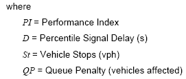
6.6.3 Split Distribution
The splits operate as a part of the coordinated timing plan, essentially acting as another set of maximum green times for the non-coordinated phases. Once a cycle length is determined, split distribution is the process of determining how much of the cycle should be provided to each of the phases. These are maximum durations a phase may be served before it must terminate and yield to the next phase. Splits are typically allocated to provide a design level of capacity to all of the minor movements, with the remaining residual time allocated to the coordinated movement (21).
The coordination split for a phase i, expressed in seconds, is calculated by the sum of the green, yellow and red times, gi + yi + ri. A split for phase i, expressed as a percentage, is calculated as 100(gi + yi +ri)/C. This gi value is independent of the maximum green time for phase i and the walk and flashing don’t walk (if applicable). The actuated logic described in Chapter 5 applies to the phase and thus the phase may not use the entire split percentage allocated within the cycle. Figure 6-21 shows these three timers, the basic timing parameters for vehicles and pedestrians and the corresponding split time associated with the coordination plan. The coordinated phase is slightly different in this regard, in that it receives the remaining time available in the cycle length.
Determining adequate split times can be challenging. If a split time is too long, other approaches may experience increased delays, while if a split time is too short, the demand may not be served. There are often opportunities to vary controller parameters to allow for the fluctuations in daily traffic flow. As shown in Figure 6-21, there are many factors that should be considered in developing signal timing for both a single and a series of intersections.
Figure 6-21 How a phase times
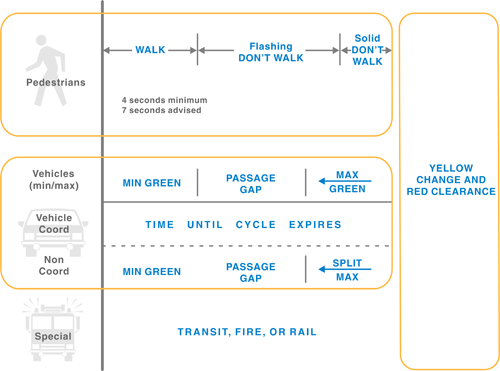
Maximum green values may be ignored during coordination using the INHIBIT MAX feature in many controllers. This allows the phase to extend beyond its normal maximum green value.
There are various policies for determining the necessary split time for a movement. The intent with split times is to provide sufficient time to avoid oversaturated conditions for consecutive cycles, but over the course of an analysis period (15 minutes or one hour) split distributions seek to provide a volume to capacity ratio that is consistent with the operating agency’s design standards. In many cases, this will provide an opportunity for fluctuations to be met with the slack time or variable green time, and the actuated operation will reduce phases as necessary to maintain efficient operations. Slack time is defined as the additional time in a cycle that is more than the minimum split times for the phases at the intersection. One common policy allocates the green time such that the volume to capacity ratios for the intersection critical movements are equal in the coordinated cycle length. Another policy is to allocate a minimum amount of time to the minor streets and the remainder to the major or coordinated phases to enhance progression opportunities and maximize bandwidth. The latter methodology is used in traditional coordination, assuming the non-coordinated phases gap out. With many controller parameters and features, this allocation of green time can depend on pedestrians, transit phases, and gap settings.
Coordinated Phase
The length of the coordinated phase split is defined by the demand on the other movements. The coordinated phase receives the time within the cycle that is unused by the other phases of each ring.
There is a close relationship between the rings with the barrier on the intersecting street and therefore the various movements must be considered carefully. In periods of low demand on the non-coordinated phases, the coordinated phase may receive the entire cycle in the absence of an opposing call. The opposing call must be received before the permissive window expires.
Non-Coordinated Phase(s)
For a non-coordinated phase to time during a cycle, a call must be active, or the phase could be activated if a corresponding phase in the other ring is active and dual entry is enabled. For instance, if phase 4 has an active call, the last movement (phase 8 is most likely) will be green as long as phase 4 is active and dual entry is enabled for phase 8. Once the phase is active the basic signal timing settings (described in Chapter 5) and the split defined in the coordination plan determine the length of the phase.
6.6.4 Offset Optimization
Offsets should consider the actual or desired travel speed between intersections, distance between signalized intersections, and traffic volumes. In an ideal coordinated system, platoons leaving an upstream intersection at the start of green should arrive at the downstream intersection near the start of the green indication. For the users, this is a relative offset, where the time-distance relationship is observable and promotes progression. The actual offset is not always observable because of the actuated logic within the controller that can provide an early return to green.
The HCM suggests that an analyst should review the time-space diagrams to analyze arterial progression and the effectiveness of offsets for a set of signal timing plans. The actuated coordination logic of each signal controller causes the green time allocated to the side street to vary on a cycle by cycle basis. Thus, the time-space diagram is dynamic because of the phenomenon of “early return to green” that results from variable demand on the non-coordinated phases. The HCM translates this assessment of offsets into an arrival type that is used to modify the second delay term of the delay equation. Determining the quality of progression factor (PF) term of the HCM average intersection delay equation is a difficult task, even if observed in the field. In fact, a study where traffic engineers were asked to observe several identical video clips of vehicles arriving at a traffic signal indicating those subjective assessments had wide ranges in estimated arrival types.
Traditional methods for field optimization have included an engineer or technician observing in the field to determine whether the timing plan is operating and whether the offsets are effectively progressing traffic between intersections. These observations provide the engineer or technician with a limited ability to review conditions. With a 100-second cycle, there are 36 cycles during an hour, and the effect of an early return to green on one cycle may not be indicative of the next cycle’s performance. Assuming an observation period of at least three cycles leads the field performance assessment with a limited review of the conditions. Engineers are supplementing the field review with improved data.
6.7 COORDINATION COMPLEXITIES
This section discusses the various complexities of signal coordination. There are many variables that that must be considered to achieve an acceptable coordination plan. The guidelines address the following topics:
- Hardware limitations
- Pedestrians
- Phase sequence
- Early return to green
- Heavy side street volumes
- Turn bay interactions
- Oversaturated conditions 6-38
Each of these topics is addressed separately in the remainder of this section.
6.7.1 Hardware Limitations
The microprocessor-based traffic signal controllers used today allow vendors to add new features by changing firmware or software. Advancements in processing power have led to many developments (e.g., alternative phase sequences, number of available timing plans, etc) as well as a variety of signal timing practices. The incompatibility of the equipment and various functionalities has led to some frustration for maintenance personnel. Various government agencies and the National Electrical Manufacturers Association have been actively developing standards to address some of the inconsistencies in hardware.
Although the actual traffic signal system technology and standards have evolved significantly in recent years, many issues such as funding, political support, management, training, inter-jurisdictional coordination, and common regional visions for system operation have significant opportunities for improvement (22). Limitations of funding to upgrade older traffic signal controllers have led to systems that meet today’s needs, but “do not provide the building blocks for cost-effectively implementing integrated and interoperable systems.” (23).
A particular example of this, as it relates to coordination, is the use of various cycle lengths throughout a day and during different times of the year. It is conceivable that a different set of timing plans is needed for summer and winter months (associated with tourist or other traffic trends), and five different timing plans are desired during a typical weekday and five additional plans warranted on the weekend. This may require the traffic signal controller to operate 20 different plans, which may not be possible due to memory storage in older versions of the hardware.
6.7.2 Pedestrians
Pedestrian operations can have a direct impact on the ability to maintain coordination along an arterial. For some agencies, pedestrian crossing time is provided for all coordination plans within the split time for the phase, while other agencies (and controllers) allow traffic signals to suspend coordination when there is a pedestrian call, requiring the controller to resynchronize after a pedestrian call. Providing for pedestrian crossing time every cycle may result in a larger cycle and a reduction in green time available for main street movements. This may result in a less than optimal timing plan.
The provision of pedestrian timing and the effects of that pedestrian timing on coordination are two distinct concepts. Pedestrian timing is required for all phases that serve pedestrians. However, when pedestrian activity is relatively low, it may be desirable to allow a pedestrian call to have an impact on coordination because the network system is more efficient without accommodating pedestrians within the coordinated cycle length.
Pedestrian timing for non-coordinated phases
The effect of pedestrian timing on coordination is most commonly seen as it affects minor street timing. Figure 6-22 illustrates the basic principle of pedestrian timing for the minor street where the vehicle split is sufficient to accommodate the required pedestrian time.
Figure 6-22 Non-coordinated phase operation with pedestrian timing completed before the force-off for that phase.
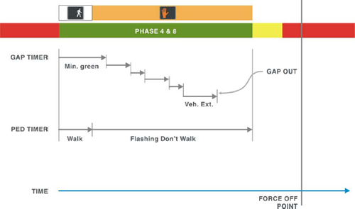
When the split for the phase in question is not sufficient to cover the pedestrian timing, the controller times the phase beyond its force-off point, as illustrated in Figure 6-23. The response of the controller depends on a two factors: (1) demand for subsequent non-coordinated phases and (2) non-actuated versus actuated operation for the coordinated phases.
Figure 6-23 Non-coordinated phase operation with pedestrian timing exceeding phase split
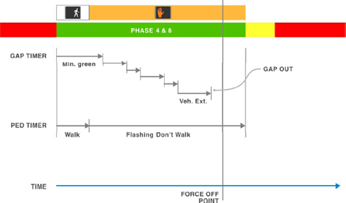
When the coordinated phases are non-actuated, the coordinated phases must begin timing sufficiently in advance of the controller’s yield point to enable full vehicle timing (minimum green) and pedestrian timing (walk plus flashing don’t walk). Should the amount of time be insufficient to cover these timing requirements, the controller will time the coordinated phase past the yield point and fall out of coordination, as shown in Figure 6-24. It is at the yield point that the controller logic determines the method by which the controller will transition back into coordination.
Figure 6-24 Loss of coordination due to pedestrian call
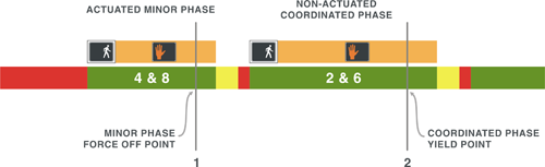
As a general rule, it is desirable to accommodate pedestrian timing entirely within the split for a given phase. By doing so, any pedestrian calls that may occur can be accommodated without causing the controller to time the phase beyond its force-off point. In these circumstances, the controller loses coordination and must transition back into coordination.
In practice, it is possible to use smaller splits than are needed to cover pedestrian timing without adversely affecting coordination. The ability to do this depends on the capability of the controller. For example, using one particular brand of controller, coding vehicle split times of 85 to 90 percent of the pedestrian timing (walk plus flashing don’t walk plus vehicle clearance interval timing) results in an immediate loss of coordination. In other cases, when these force-offs are combined with cycle lengths that are long enough to allow a controller to temporarily shorten its cycle length during transition without violating the controller minimum (typically at least 10 percent greater than the controller minimum cycle length), the controller will typically resynchronize within a cycle or two, thus having minimal adverse effect on coordination.
A questionnaire survey from the NCHRP 172 project (24) indicated that as a general rule, pedestrian minimum time should be used for the side street when a pedestrian call occurs more than 20 percent of the cycles.
Pedestrian timing for coordinated phases
The amount of time needed to serve vehicle volume or provide bandwidth along the major street usually results in coordinated phase splits that are sufficient to accommodate pedestrian timing. Many controllers require that pedestrian timing be accommodated within the coordinated split timing to allow any type of coordinated operation.
For controllers operating with non-actuated coordinated phases, the major street splits must be large enough to accommodate all vehicle and pedestrian minimum timing requirements. For actuated coordinated phases, however, it is sometimes possible to provide a split for the coordinated phases that is less than that required to serve pedestrians. In practice, this works acceptably only if (1) pedestrian demand along the major street results in relatively few pedestrian calls, and (2) demand for the non-coordinated phases is frequently less than the split. In these cases, the controller can take advantage of the unused time from the non-coordinated phases to serve the coordinated pedestrian timing without passing the yield point and falling out of coordination.
6.7.3 Phase Sequence
The sequence of phases, particularly those of left turns, can provide measurable benefit to arterial operation. The most common phase sequencing decision, whether to lead or lag left turns, can have a particularly strong impact on the ability to provide bandwidth in both directions of an arterial. Other phase sequence decisions, such as the sequence of left turns on the minor street or the sequence of split phasing on the minor street, do not directly impact arterial bandwidth but can affect arterial delay. These two concepts are discussed in the following sections.
Major street left-turn phase sequence
Modern controllers allow left turn phase sequences to be varied by time of day. This has traditionally been done only for protected left-turn operations, but the use of specific display techniques allows this to be extended to protected-permissive operations (see Chapter 4).
The basic concept of lagging a major street left turn is to time the left turn after the opposing through movement (assumed to be one of the coordinated phases) terminates. Figure 6-25 illustrates a typical time-space diagram showing an arterial with only leading lefts and the same arterial with both leading and lagging lefts. The arterial demonstrated in the figure has a major intersection on each end and a minor intersection in the middle. As can be seen in the figure, a lagging left turn at the middle intersection facilitates better progression in both directions because it allows the two platoons to arrive at different times in the cycle. In addition, the two major intersections benefit to some degree from selective lagging left turns.
Figure 6-25 Vehicle trajectory diagrams showing the effect of changes in phase sequence
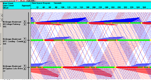
Figure 6-25a is a vehicle trajectory diagram for an arterial with only leading left turns on the major street.
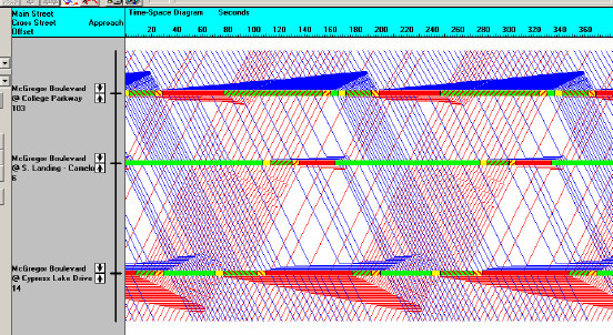
Figure 6-25b is a vehicle trajectory diagram for the same arterial but using selective lagging left turns on the major street.
One of the potential consequences of lagging left turns that are actuated is that the end of the adjacent coordinated phase becomes less predictable. In terms of dual-ring operation, the lagging left turn is typically served after the deterministic (yield) point is reached. The lagging left turn extends the concurrent (adjacent) through movement time indirectly, not as a result of any particular timing within the coordinated phase itself. As a result, only the detection for the lagging left turn is used to determine when to gap out the lagging left turn phase and the adjacent coordinated phase. Therefore, it is possible that the adjacent coordinated phase may gap out earlier than expected from cycle to cycle.
One technique that has been used to eliminate this variability is to use a maximum recall on the lagging left-turn phase. In most controllers, this can be set by time of day and can often be paired with the specific timing plan containing the lagging left turn. The use of a maximum recall on the lagging left turn makes the end of the adjacent coordinated phase more predictable. On the other hand, if the demand for the lagging left turn is highly variable or is less than the split coded, the use of the recall on the lagging left turn may give the appearance of sluggish operation or defective detection.
In addition to the operational differences associated with lagging left turns, some have expressed concern over potential safety differences with having left turn sequencing changing by time of day. Even if lagging operation is used during coordinated operation during the majority of the day, the intersection is often configured to revert to leading-left operation when operating free (uncoordinated) during nighttime operations. There is no definitive research offering consensus on whether changing the left-turn sequence throughout the day has any negative safety consequences.
Minor-street phase sequence
It may be advantageous in some circumstances to adjust the left-turn phase sequence for the minor street. In doing this, it may be possible to reduce the delay and queuing for minor-street left turns as they enter the major street and arrive at downstream intersections. Although such adjustments may affect system-wide delays and stops, they will have no effect on the theoretical bandwidth for the coordinated phases.
6.7.4 Early Return to Green
One of the consequences of coordinated, actuated control is the potential for the coordinated phase to begin earlier than expected. This “early return to green” occurs when the sum total of the time required by the non-coordinated phases is less than the sum total of the vehicle splits coded for the phases. While this may reduce delay at the first intersection, it may increase system delay because of inefficient flow at downstream intersections or, most important, the critical intersection of the network. Figure 6-26 illustrates this within a time-space diagram.
Figure 6-26 Time-Space Diagram Example of Early Return to Green
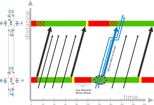
Figure 6-26 shows that vehicles in coordinated phases that begin early may be forced to stop at one or more downstream intersections until they fall within the “band” for that direction of travel. This can result in multiple stops for vehicles and a perception of poor signal timing.
Early return to green can have a substantial negative effect on the performance of the coordinated phases. Research for offset transitioning has been completed to “smooth progression of a platoon through an intersection using the volume and occupancy profile of advance detectors” (25). Early return to green can be difficult to manage along a corridor, and it rarely can be completely prevented without eliminating most of the benefits of actuation. One technique that is sometimes used is to delay the start (offset shifted to the right) of the coordinated phase at a critical upstream intersection with sufficient non-coordinated demand (thus making its operation more predictable). Similarly, minor intersections downstream of this critical offset can be started earlier (offset is shifted left in a time-space diagram) to minimize the likelihood of a stop due to an early return to green. In either case, the engineer should use caution when shifting offsets to address early return to green in one direction may adversely affect operation in the opposite direction.
6.7.5 Heavy Side Street Volumes
Heavy side street volumes can affect the ability to progress through movements along an arterial. These volumes can come from either signalized intersections within the coordinated signal system or from unsignalized intersections, or from driveways between coordinated signals. Interchanges are a common source of heavy side street volumes.
In many cases, this additional demand proceeds along the remainder of the arterial and becomes part of the major street through demand at downstream intersections. However, this demand often enters the system outside the band established for through movements traveling end-to-end along the arterial. It is usually desirable to adjust downstream intersection timing to allow these heavy side street movements to proceed with a minimum of stops. In these cases, solutions that seek to optimize arterial bandwidth may be counterproductive to effective signal timing.
6.7.6 Turn Bay Interactions
Turn bay (or turn pocket) interactions can significantly reduce the effective capacity of an intersection. This is experienced when either demand for the turning movement exceeds the available storage space or when vehicle queues block the entrance of a turn bay. If left-turn demand cannot enter the left-turn bay due to impeding through vehicles, the left-turn phase will gap out early due to a perceived lack of demand. This results in some left turning traffic requiring more than one cycle to be served. In addition, the through movements lose capacity due to the impedance of left turns. In some cases, this may effectively remove an entire through lane from being able to effectively serve through demand.
Turn bay overflows also adversely impact progression. The impedance created by left-turn vehicles stored in the through lane prevents through traffic from proceeding to downstream intersections. As a result, any platoon of through vehicles passing through the affected intersection tends to be dispersed. This reduces the ability for downstream intersections to efficiently provide green time for the platoon.
Turn bay overflows can occur under both under- and oversaturated conditions. Even if enough green time is provided to serve a given turning movement, turn bay overflow can occur if the available storage is insufficient to store the queue for a given cycle. For cases where the turn bay is fed from a two-way left-turn lane, turn bay overflow rarely has significant adverse consequences for the adjacent through movements. For locations with raised medians, on the other hand, turn bay overflow can result in left-turning vehicles extending into the adjacent through lane.
Turn bay overflow can be managed in a number of ways:
- Turn bays can be extended to accommodate the necessary storage. This is typically the best solution, but it may be infeasible due to physical constraints, access needs, turn bay requirements for adjacent intersections, or other factors.
- Shorter cycle lengths can be used to keep overall queue lengths shorter, thus reducing the likelihood of overflow or turn bay blocking.
- If the left turn is protected, protected-permissive left-turn phasing may be considered to allow some of the left turn demand to be processed during the permissive portion of the phase. This reduces the overall queue length.
- If the left turn is permissive, protected-permissive left turn phasing may be considered to provide a period of higher saturation flow rates (the protected portion of the phase). This technique, however, may result in longer cycle lengths that partially offset the gain in capacity. Some agencies use a lagging protected period after the permissive period that is called only if there remains any unserved left-turn demand at the end of the permissive portion of the phase.
- Conditional service for the phase may be invoked, bringing up the movement twice during the cycle.
- If two receiving lanes are available, the adjacent through lane can be designated as a shared left-through lane and the phasing changed to split phasing. While this is rarely desirable for major street movements, it may be an appropriate solution for minor street movements.
- At an intersection with one heavy left-turn movement on the major street, it may be preferable to designate the left-turn phase as one of the coordinated movements paired with the adjacent through movement (e.g., phases 1 and 6 or phases 2 and 5). This allows any unused time to roll over to the left-turn phase of interest, thus reducing its effective red time and associated queue formation.
6.7.7 Critical Intersection Control
A challenging aspect of timing an arterial street or a network of streets is the need to provide enough capacity for major intersections without creating excessive delay for minor intersections. Ideally, all of the intersections to be coordinated operate optimally with similar cycle lengths. However, most arterial streets do not have this optimal arrangement due to a mixture of simple signals (e.g., two phases) with more complex signals (e.g., eight phases), wide ranges in cross street volume (e.g., major arterials versus collectors), and variations in left-turning volumes.
The techniques to determine the ideal cycle length for each intersection in isolation were covered earlier. The critical system cycle length is the maximum optimal cycle length of any intersection in the system.
Several techniques can be used where there is a significant disparity in the ideal cycle length for each intersection:
- Each intersection is timed using the critical system cycle length. This ensures the ability to coordinate all of the intersections in the system. However, it may result in excessive delay at minor intersections.
- Each intersection is timed to either the critical system cycle length or to half that value. This technique is commonly referred to as “double cycling” (a minor intersection cycles twice as frequently as a major intersection) or “half cycling” (a minor intersection has half the cycle length of the major intersection). This method can often produce substantially lower delays at the minor intersections where double cycling is employed. However, it may become more difficult to achieve progression in both directions along the major arterial, which may result in more arterial stops than desired.
- The major intersections are operated free, and the minor intersections are coordinated using a shorter cycle length. Because the major intersections are operating free, it is impossible to provide coordination through the major intersections. Therefore, major street vehicles are likely to stop at both the major intersection and at a downstream intersection due to randomness in arrival at and departure from the major intersection. This technique can often result in lower overall system delay at the expense of additional stops along the major street.
6.7.8 Oversaturated Conditions
Timing for oversaturated conditions requires different strategies than those used for undersaturated conditions. An intersection that is operating at or over capacity requires all movements to operate at a saturation flow rate to serve demand. Beyond this, the timing plan may favor the movements with the most lanes to maximize the throughput of the intersection. Obviously, the timing plan must consider whether undesirable effects such as turn bay overflow or other conditions exacerbate the problem.
Under these conditions, arriving vehicles must join the back of a queue to ensure that they enter the intersection with a minimum amount of headway (maximum saturation flow rate); however, it is impossible for vehicles on the arterial to maintain a travel speed traditionally desired for coordination.
In addition, an oversaturated approach cannot serve all arriving demand, thus creating a residual queue at the end of a cycle that carries over to subsequent cycles. This residual queue depends on demand conditions and can grow from cycle to cycle. Even when demand drops, the residual queues create saturated conditions beyond the time period when the arriving demand would create saturated conditions by itself. These residual queues can extend to adjacent intersections and prevent traffic from exiting upstream intersections if the intersections are closely spaced.
The general technique for accommodating oversaturated conditions involves managing queues. The following sections present options available for accommodating oversaturated conditions, including benefits and trade-offs.
Queue storage on minor movements to favor major movements
It is sometimes possible to accommodate oversaturated conditions by favoring the coordinated movements at the expense of minor street movements. Under this strategy, the coordinated phases are timed for a volume-to-capacity ratio typically no higher than 0.95 to 0.98. The minor movements receive less green time, which results in demand-to-capacity ratios exceeding 1.0. This method has a few advantages. The major street receives priority, which helps maintain traffic flow along the major street. This typically benefits the heaviest movements through the intersection, as well as the transit and emergency vehicles who frequently use the major street. In addition, demand held on side streets cannot enter downstream intersections, thus improving the actual downstream flow rate.
However, this type of timing strategy can have significant disadvantages. While this method can theoretically keep the major street moving, it creates extensive delay and queuing on side streets. This can have negative safety repercussions and highly negative public feedback. More importantly, it may be impossible to reduce splits for side-street through movements due to pedestrian timing requirements. If pedestrian calls are frequent enough to cause the side street through movement to time to its full split, the only movements with time available for use are the major street left turns and the minor street left turns (if present). Queue spillback for the major street left turns can exceed available storage and spill into the adjacent through movement, creating operational and safety problems. As a result of these disadvantages, this technique is often not desirable.
Use of short cycle lengths
One of the most effective techniques in managing oversaturated conditions is the use of shorter cycle lengths. Shorter cycle lengths allow more frequent servicing of all movements at only a minor expense of additional loss time during the peak time period. This frequent cycling provides more equitable servicing of all movements and allows drivers to visibly experience progress, even if it takes multiple cycles to be served at a given intersection.
Queue management on major street movements
An alternative technique is to selectively store queues on major street movements. Candidates for this treatment frequently include major intersections that are spaced far enough from other signalized intersections to allow the queues to grow without creating upstream intersection impacts. In addition, drivers may be more accepting of congestion at major intersections than at minor intersections.
For network applications (e.g., downtown grids), it is often best to store queues outside the network using key signals to meter traffic into the grid network. While this creates congestion at some intersections, it allows a network of intersections to operate undersaturated, thus enabling traffic to progress through the network.
Use of actuated uncoordinated operation
Removing the cycle length constraint during the oversaturated period can result in efficient allocation of green time, provided gap timers are set appropriately. There are emerging strategies such as lane-by-lane detection and measurement of flow used as opposed to presence for control logic decision-making and operation.
6.8 REFERENCES
- National Traffic Signal Report Card, National Transportation Operations Coalition, 2005.
- Fundamentals of Traffic Engineering (15th ed.), UCB-ITS-CN-01-1, January 2001
- Srinivasa R. Sunkari, Roelof J. Engelbrecht, and Kevin N. Balke, Evaluation Of Advance Coordination Features In Traffic Signal Controllers
- Albert Grover & Associates, “Minimize Delay, Maximize Progression with Protected Permissive Lead/Lag Phasing”, Technical Workshop. Inland Empire Section of ITE, December 14, 1995.
- Frederickson, J. Letter to the Arizona Insurance information association. October 2000.
- Kittelson & Associates, Evaluation of Traffic Signal Displays for Protected/Permissive Left-Turn Control. NCHRP 3-54(2), Final Report, FHWA, U.S. Department of Transportation, Washington, DC, 2003.
- Shelby, S. G., Bullock, D. M., and Gettman, D. Transition Methods in Traffic Signal Control. Transportation Research Record: Journal of the Transportation Research Board, No. 1978, Transportation Research Board of the National Academies, Washington, D.C., 2006, pp. 130-140.
- Zong Z. Tian, Tom Urbanik, Kent Kacir, Mark Vandehey, and Howard Long, “Pedestrian Timing Treatment for Coordinated Signal Systems”, viewed at http://wolfweb.unr.edu/homepage/zongt/Publications_files/PedTimingICTTS.pdf January 17, 2007.
- Signalized Intersections Guide
- Los Angeles Department of Transportation, “Early Methods for Traffic Signal Network Timing” http://www.lacity.org/ladot/TopicsAndTales/TrafficSigTiming6.pdf March 5, 2007.
- Nelson, Eric “Timing Strategies for Managing Oversaturation in Harris County”, Presentation at the TRB Summer Meeting, Woods Hole, MA, July 11, 2006
- Lieberman, Ed, NCHRP 3-38 (4), Transportation Research Board, 1992.
- Parsonson, “Signal Timing Improvement Practices”NCHRP Synthesis 172 National Research Council, Transportation Research Board, Washington, D.C., February 1992
- Webster, F.V., “Traffic Signal Settings,” Road Research Technical Paper No. 30, HMSO, London (1958)
- Teply, Stan “Saturation Flow at Signalized Intersections through a Magnifying Glass,”Proceedings of the Eight International Symposium on Transportation and Traffic Theory University of Toronto Press, 1983.
- Alexiadis, V. K. Jeannotte, A. Chandra, Traffic Analysis Toolbox Volume I: Traffic Analysis Tools Primer, FHWA -HRT-04-038, June 2004.
- Signal Timing Process, Federal Highway Administration, Sabra Wang, December 30, 2003
- Fambro, Sunkari, Sangineni, “Guidelines for Retiming Arterial Networks”, Texas Transportation Institute, February 1993
- Trafficware. Synchro 6 Users Manual, 2004.
- MnDOT Traffic Signal Timing and Coordination Manual, March 2005
- Bullock, D. and A. Sharma, MOST PROJECT Laboratory 6. Actuated Traffic Signal Control, DRAFT, January 2007.
- Transportation Infrastructure, Benefits of Traffic Control Signal Systems Are Not Being Fully Realized. GAO/RCED-94-105, Report to the Chairman, Committee on Energy and Commerce, House of Representatives, United States General Accounting Office, Washington, D.C., March 1994
- 23 Bullo, Darcy and Tom Urbanik, “Addressing Diverse Technologies and Complex User Needs”, http://onlinepubs.trb.org/onlinepubs/millennium/00116.pdf January 17, 2007
- Ibid
- Abbas, Montasir, Darcy Bullock, and Larry Head, “Real-time offset transitioning algorithm for coordinating traffic signals”, Transportation Research Record 1748, Washington D.C. 2001