Traffic Signal Timing Manual
Contact Information: Operations Feedback at OperationsFeedback@dot.gov
This publication is an archived publication and replaced with the Signal Timing Manual - Second Edition.
CHAPTER 3
OPERATIONAL AND SAFETY ANALYSIS
TABLE OF CONTENTS
- 3.0 Operational and Safety Analysis
- 3.1 Terminology
- 3.2 Characteristics Affecting Signal Timing
- 3.2.1 Location
- 3.2.2 Transportation Network Characteristics
- 3.2.3 Intersection Geometry
- 3.2.4 User Characteristics
- 3.3 Capacity and Critical Movement Analysis
- 3.3.1 Basic Operational Principles
- 3.3.2 Saturation Flow Rate
- 3.3.3 Lost Time
- 3.3.4 Capacity
- 3.3.5 Volume-to-Capacity Ratio
- 3.3.6 Critical Movement Analysis
- 3.4 Intersection-Level Performance Measures and Analysis Techniques
- 3.4.1 Performance Measures
- 3.4.2 Evaluation Techniques: The HCM Procedure for Signalized Intersections
- 3.4.3 Practical Operational Approximations
- 3.4.4 Intersection-Level Field Measurement
- 3.5 Arterial- and Network-Level Performance Measures and Prediction Techniques
- 3.5.1 Arterial- and Network-Level Performance Measures
- 3.5.2 Evaluation Techniques
- 3.5.3 Arterial and Network Field Measurement Techniques
- 3.6 Safety Assessment
- 3.6.1 Crash Data Review
- 3.6.2 Quantitative Safety Assessment
- 3.7 Signal Warrants
- 3.8 References
LIST OF TABLES
- Table 3-1 Steps of the Quick Estimation Method (QEM) (2, with HCM corrections)
- Table 3-2 Volume-to-capacity ratio threshold descriptions for the Quick Estimation Method
- Table 3-3 Motor vehicle LOS thresholds at signalized intersections
- Table 3-4 Planning-level cycle length assumptions
- Table 3-5 HCM arterial class definitions
- Table 3-6 Arterial level of service
- Table 3-7 Guidelines for bandwidth efficiency
- Table 3-8 Guidelines for bandwidth attainability
- Table 3-9 Evaluation Techniques for Performance Measures
- Table 3-10 Summary of crash types and possible signal modifications to benefit safety
LIST OF FIGURES
- Figure 3-1 Effect of intersection skew on signalized intersection width
- Figure 3-2 Figure 3-2 Typical flow rates at a signalized movement
- Figure 3-3 Illustration of volume and capacity of a signalized movement
- Figure 3-4 Overview of signalized intersection analysis methods
- Figure 3-5 Graphical summary of Critical Movement Analysis/Quick Estimation Method (1)
- Figure 3-6 Sample travel time run result graph
3.0 OPERATIONAL AND SAFETY ANALYSIS
The purpose of this chapter is to summarize some of the common techniques used to assess the operational and safety performance of signal timing. The chapter begins by presenting an overview of the characteristics that affect signal timing, including both system and user characteristics. It then presents discussions of operational and safety performance measures and techniques to evaluate those performance measures. Finally, the chapter presents a discussion of signal warrants as presented in the Manual on Uniform Traffic Control Devices and how those warrants relate to signal timing.
3.1 TERMINOLOGY
This section identifies and describes basic terminology used within this chapter. Additional terms can be found in the Glossary section of the Manual.
Capacity
The maximum rate at which vehicles can pass through the intersection under prevailing conditions.
Clearance lost time
The time, in seconds, between signal phases during which an intersection is not used by any critical movements.
Control Delay
The amount of additional travel time experienced by a user attributable to a control device.
Critical movement analysis
A simplified technique for estimating phasing needs and signal timing parameters.
Delay
The additional travel time experienced by a driver, passenger, or pedestrian.
Effective green time
The time during which a given traffic movement or set of movements may proceed; it is equal to the cycle length minus the effective red time.
Flow rate
The equivalent hourly rate at which vehicles, bicycles, or persons pass a point on a lane, roadway, or other trafficway, computed as the number of vehicles, bicycles, or persons passing the point, divided by the time interval (usually less than 1 hour) in which they pass; expressed as vehicles, bicycles, or persons per hour.
Level of service
A qualitative measure describing operational conditions within a traffic stream, based on service measures such as speed and travel time, freedom to maneuver, traffic interruptions, comfort, and convenience.
Lost Time
The portion of time at the beginning of each green period and a portion of each yellow change plus red clearance period that is not usable by vehicles.
Saturation Flow Rate
The equivalent hourly rate at which vehicles can traverse an intersection approach under prevailing conditions, assuming a constant green indication at all time and no loss time, in vehicles per hour or vehicles per hour per lane.
Start-up lost time
The additional time, in seconds, consumed by the first few vehicles in a queue at a signalized intersection above and beyond the saturation headway due to the need to react to the initiation of the green phase and to accelerate to a steady flow condition.
Stopped Delay
A measurement of the aggregate sum of stopped vehicles for a particular time interval divided by the total entering volume for that movement.
Total delay
The sum of all components of delay for any lane group, including control delay, geometric delay, and incident delay.
Travel Time (Average)
The total elapsed time spent traversing a specified distance. The average travel time represents an average of the runs for a particular link or corridor.
3.2 CHARACTERISTICS AFFECTING SIGNAL TIMING
Several overall features affect implementation of signal timing including:
- Location
- Transportation network characteristics
- Intersection geometry
- User characteristics
The following sections further describe many characteristics and dynamic nature influencing signal timing.
3.2.1 Location
One of the primary factors affecting overall signal timing is the environment in which the intersection or intersections being timed are located. Urban environments are frequently characterized by lower speeds and higher degrees of congestion. In addition, urban environments are frequently characterized by higher pedestrian, cyclist, and transit use that often require priority in consideration. Rural environments, on the other hand, are typically higher speed but with lower levels of traffic volumes and fewer, if any, pedestrians, cyclists, and transit vehicles. As a result, signal timing for rural environments is typically dominated by efforts to safely manage high speed approaches; capacity is seldom a constraint. Suburban environments often present a challenging mix of these characteristics. Suburban environments are often characterized by high speeds during the off-peak periods and capacity-constrained conditions during the peak periods. This requires a careful consideration and balance of both safety aspects and operational efficiency.
3.2.2 Transportation Network Characteristics
The configuration of the transportation network under consideration can have a significant impact on the way its traffic signals are timed. Isolated intersections can be timed without the explicit consideration of other traffic signals, allowing the flexibility to either set or target cycle lengths that are optimal for the individual intersection. In these cases, good detection design often yields measurable operational and safety benefits. These are discussed further in Chapters 4 and 5.
For intersections located along arterial streets, isolated operation can often be improved by considering coordination of the major street movements along the arterial. Common cycle lengths are often employed to facilitate this coordination. Coordinated operations are discussed in detail in Chapter 6.
Signalized intersections are often located in grid networks with either crossing arterials or a series of intersecting streets with comparable function and traffic volumes. In these cases, the entire network is often timed together to ensure consistent behavior between intersections. Grid networks, particularly downtown environments with short block spacing, are frequently timed using fixed settings and no detection.
Within these categories, the spacing of signalized intersections affects how one times the signals. For signals that are sufficiently far apart that they can be considered independent of one another, intersections may be operated freely without need for or benefit from coordination, depending on the degree of congestion on the facility. For most arterial streets with signal spacing between 500 feet and 0.5 mile (2,640 feet), coordinated operation can often yield benefits by improving progression between signals. On arterials with higher speeds, it can be beneficial to coordinate signals spaced a mile (5,280 feet) apart or even longer. Signals that are located very close together (less than 500 feet) often require settings that manage queues rather than progression as the dominant policy. It may also be beneficial to operate two intersections with very close spacing with a single controller.
3.2.3 Intersection Geometry
The overall geometry of an intersection determines its ability to efficiently and safely serve user demand. Pedestrians are often crossing lanes of traffic, whereas transit, bicycles, and vehicular traffic are using the travel lanes provided at the intersection. The number of lanes provided for each approach has a significant impact on the capacity of the intersection and, therefore, the ability for signal timing to efficiently serve demand. For example, a movement served by two lanes rather than one has a higher capacity and thus requires less green time to serve demand. However, increasing the number of lanes on a particular leg of the intersection also increases the minimum pedestrian crossing time across that leg, which by increasing clearance times will offset some of the increase in capacity.
Subtle details of intersection geometry have a significant influence on signal timing. The size and geometry of the intersection, coupled with the speed of approaching vehicles and walking pedestrians, affect vehicular and pedestrian clearance intervals, which in turn have an effect on the efficiency of the intersection’s operation. For example, the skew of an intersection (the angle at which two roadways intersect) influences the length of crosswalks and thus pedestrian clearance time. The crosswalk length for an intersection at right angles (90 degrees) with a crosswalk length of 61 feet can extend to 76 feet if the intersection is skewed to 60 degrees, as shown in Figure 3-1 below. If a pedestrian walking speed of 4.0 ft/s, for example, is used for pedestrian clearance interval timing, the skew increases the pedestrian clearance interval from 16 seconds to 19 seconds; for a pedestrian walking speed of 3.5 ft/s, the clearance interval increases from 18 seconds to 22 seconds. Reverse effects can be seen when smaller curb radii and/or curb extensions are used to shorten pedestrian crosswalks, thus reducing pedestrian clearance time requirements (1). Although curb extensions can shorten pedestrian crossing times, the resulting narrow width may restrict the ability for through vehicles in shared lanes to bypass right-turning vehicles that are waiting for pedestrians or left-turning vehicles waiting for gaps in opposing traffic.
Regardless of the angle of skew, care should be taken to ensure that good visibility of the signal heads is maintained for approaching vehicles.
Figure 3-1 Effect of Intersection skew on signalized intersection width
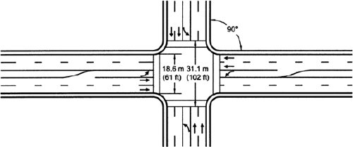
Figure 3-1 illustrates the impact of skewed intersection geometry on signal operations. As the angle between two typical four lane intersecting arterials decreases from 90 degrees, to 75 degrees, and then to 60 degrees, the crosswalk lengthens from 61 feet, to 63 feet, and then to 76 feet respectively. The greater the skew, the greater the pedestrian crosswalk distance, resulting in longer clearance times.Intersection skew at 90 degrees.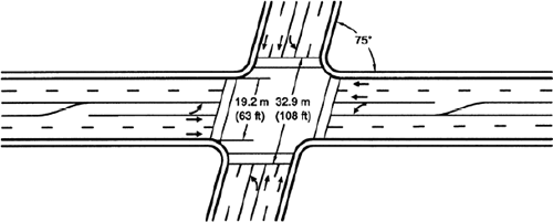
Intersection skew at 75 degrees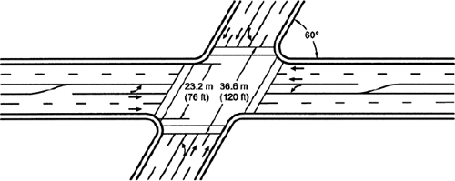
Intersection skew at 60 degrees.
Source: Figure 15, FHWA Signalized Intersections: Informational Guide
3.2.4 User Characteristics
User characteristics clearly influence the effectiveness of signal timing and should be accounted for early in the planning and analysis process. Some of the important factors include the following:
- Mix of users: The mix of users at an intersection has a significant influence on signal timing. Pedestrians with slower walking speeds, persons using wheelchairs, and pedestrians with visual impairments need more time to cross the street; pedestrian walk times and clearance intervals need to be adjusted accordingly. High bicycle use may benefit from special bicycle detection and associated bicycle minimum green timing. Emergency vehicle and/or transit use may justify the use of preemption and/or priority. Truck traffic requires accounting for reduced performance (longer acceleration and deceleration times) and larger size of heavy vehicles.
- User demand versus measured volume: Traffic demand represents the arrival pattern of vehicles at an intersection (or the system, if one considers a group of intersections together), while traffic volume is the measured departure rate from the intersection. If more vehicles arrive for a movement than can be served, the movement is considered to be operating over capacity (oversaturated). However, unless the analyst has measured demand arriving at the intersection through either queue observation or through measurement of departure rates from an upstream undersaturated intersection, the true demand at an intersection may be unknown. This can cause problems when developing signal timing plans for a given intersection, as one may add time to a given movement, only to have it used up by the latent demand for that movement. Traffic volume at an intersection may also be less than the traffic demand due to an overcapacity condition at an upstream signal that “starves” demand at the subject intersection. These effects are often best analyzed using microsimulation.
3.3 CAPACITY AND CRITICAL MOVEMENT ANALYSIS
An important principle behind effective signal timing is a basic understanding of how signal timing affects the capacity of the intersection. Capacity is discussed in detail in the Highway Capacity Manual (2), but often only the basic elements are particularly relevant to practical signal timing implementation. This section presents a discussion of the operation of a signalized intersection movement, the definition of capacity and its component elements, and a discussion of techniques to estimate capacity.
3.3.1 Basic Operational Principles
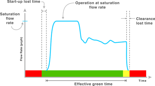
The basic operation of vehicular movement through a signalized intersection is presented in Figure 3-2 below. The signal display is presented on the horizontal axis, the instantaneous flow of vehicles on the vertical axis. During the time while the movement is receiving a red indication, vehicles arrive and form a queue, and there is no flow. Upon receiving a green indication, it takes a few seconds for the driver of the first vehicle to recognize that the signal has turned green and to get the vehicle in motion. The next few vehicles also take some time to accelerate. This is defined as the start-up lost time or start-up delay and is commonly assumed to be approximately 2 seconds. After approximately the fourth vehicle in the queue, the flow rate tends to stabilize at the maximum flow rate that the conditions will allow, known as the saturation flow rate. This is generally sustained until the last vehicle in the queue departs the intersection. Upon termination of the green indication, some vehicles continue to pass through the intersection during the yellow change interval; this is known as yellow extension. The usable amount of green time, that is, the duration of time between the end of the start-up delay and the end of the yellow extension, is referred to as the effective green time for the movement. The unused portion of the yellow change interval and red clearance interval is called clearance lost time.
Figure 3-2 Typical flow rates at a signalized movement
3.3.2 Saturation Flow Rate
The saturation flow rate, s, is an important parameter for estimating the performance of a particular movement. Saturation flow rate is simply the headway in seconds between vehicles moving from a queued condition, divided into 3600 seconds per hour. For example, vehicles departing from a queue with an average headway of 2.2 seconds have a saturation flow rate of 3600 / 2.2 = 1636 vehicles per hour per lane. Saturation flow rate for a lane group is a direct function of vehicle speed and separation distance. These are in turn functions of a variety of parameters, including the number and width of lanes, lane use (e.g., exclusive versus shared lane use, aggregated in the HCM as lane groups), grades, and factors that constrain vehicle movement such as presence or absence of conflicting vehicle and/or pedestrian traffic, on-street parking, and bus movements. As a result, saturation flow rates vary by movement, time, and location and commonly range from 1,500 to 2,000 passenger cars per hour per lane (2). The HCM provides a series of detailed techniques for estimating and measuring saturation flow rate. It should be noted that this is significantly different than the ideal saturation flow rate, which is typically assumed to be 1,900 passenger cars per hour per lane.
The ideal saturation flow rate may not be achieved (observed) or sustained during each signal cycle. There are numerous situations where actual flow rates will not reach the average saturation flow rate on an approach including situations where demand is not able to reach the stop bar, queues are less than five vehicles in a lane, or during cycles with a high proportion of heavy vehicles. To achieve optimal efficiency and maximize vehicular throughput at the signalized intersection, traffic flow must be sustained at or near saturation flow rate on each approach. In most HCM analyses, the value of saturation flow rate is a constant based on the parameters input by the user, but in reality, this is a value that varies depending on the cycle by cycle variation of situations and users.
The HCM provides a standardized technique for measuring saturation flow rate. It is based on measuring the headway between vehicles departing from the stop bar, limited to those vehicles between the fourth position in the queue (to minimize the effect of startup lost time) and the end of the queue. The detailed procedure can be found in Chapter 16 of the HCM. For signal timing work, it is often not necessary to place heavy emphasis on this parameter due to the high degree of fluctuation in this parameter from cycle to cycle.
3.3.3 Lost Time
As noted in the previous section, a portion of the beginning of each green period and a portion of each yellow change plus red clearance period is not usable by vehicles. The sum of these two periods comprises the lost time (or loss time) for the phase. This value is used in estimating the overall capacity of the intersection by deducting the sum of the lost times for each of the critical movements from the overall cycle length. The HCM defines a default value of 4 seconds per phase for total lost time (the sum of start-up lost time and clearance lost time).
The resulting effective green time can therefore be defined as follows in Equation 3-1:
Equation 3-1

3.3.4 Capacity
At signalized intersections, capacity for a particular movement is defined by two elements: the maximum rate at which vehicles can pass through a given point in an hour under prevailing conditions (known as saturation flow rate), and the ratio of time during which vehicles may enter the intersection. These are shown in Equation 3-2 (2).
Equation 3-2

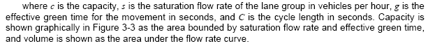
Figure 3-3 Illustration of volume and capacity of a signalized movement
For the purposes of signal timing, the factors within a practitioner’s control that directly influence capacity are somewhat limited. In most cases, the number, width, and assignment of lanes are fixed, as are grades and the presence of on-street parking and bus movements. The practitioner has some control over the effect of conflicting vehicle and/or pedestrian traffic through the use of permissive versus protected left-turn and right-turn phasing and/or exclusive pedestrian phases. For signal timing purposes, the most readily accessible parameter is the effective green time for a particular movement.
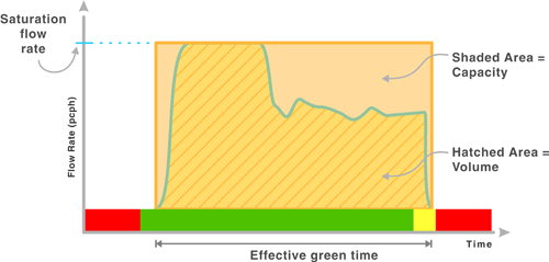
3.3.5 Volume-to-Capacity Ratio
The volume-to-capacity ratio, also known as the v/c ratio or the degree of saturation, is calculated for each movement using Equation 3-3:

where v is the demand volume of the subject movement in vehicles per hour and the remaining variables are as defined previously. Using the graphical tool from the previous section, the volume-to-capacity ratio represents the proportion of the area defining capacity that is occupied by volume.
Movements or lane groups with volume-to-capacity ratios less than 0.85 are considered undersaturated and typically have sufficient capacity and stable operations. For movements or lane groups with a volume-to-capacity ratio of 0.85 to 1.00, traffic flow becomes less stable due to natural cycle-to-cycle variations in traffic flow. The closer a movement is to capacity, the more likely that a natural fluctuation in traffic flow (higher demand, large truck, timid driver, etc.) may cause the demand during the cycle to exceed the green time for that cycle. The result would be a queue that is carried over to the next cycle, even though the overall demand over the analysis period is below capacity. In cases where the projected volume-to-capacity ratios exceed 1.00 (demand exceeding capacity) over the entire analysis period, queues of vehicles not served by the signal each cycle are likely to accumulate and either affect adjacent intersections or cause shifts in demand patterns. These conditions are described as oversaturated and require significantly different approaches for signal timing.
3.3.6 Critical Movement Analysis
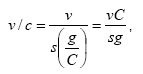
A variety of analysis procedures, ranging from simple to complex, are used to evaluate signalized intersection performance. These are summarized in Figure 3-4.
Critical movement analysis is a simplified technique that has broad application for estimating phasing needs and signal timing parameters. The most current implementation of the critical movement analysis method is provided in Chapter 10 of the HCM 2000 as the Quick Estimation Method. This method allows an analyst to identify the critical movements at an intersection; estimate whether the intersection is operating below, near, at, or over capacity; and approximate the amount of green time needed for each critical movement. The method is generally simple enough to be conducted by hand, although some of the more complicated refinements are aided considerably with the use of a simple spreadsheet. In many cases, the lack of precision of future volume forecasts or estimated trip generation of land uses minimizes the precision of more complicated analysis methods; in these cases, critical movement analysis is often as precise as one can achieve.
Critical movement analysis is based on the following fundamental basic principle:
The amount of time in an hour is fixed, as is the fact that two vehicles (or a vehicle and a pedestrian) cannot safely occupy the same space at the same time. Critical movement analysis identifies the set of movements that cannot time concurrently and require the most time to serve demand.
Critical movement analysis is an effective tool to quickly estimate green times for various movements at an intersection and to estimate its overall performance in terms of volume-to-capacity ratios. Appendix A provides step-by-step details for using the procedure, including a sample worksheet. The basic procedure for conducting a critical movement analysis/quick-estimation method analysis is given in Figure 3-5 and Table 3-1. Table 3-2 identifies the various thresholds recommended in the HCM for volume-to-capacity ratios.
Figure 3-4 Overview of signalized intersection analysis methods
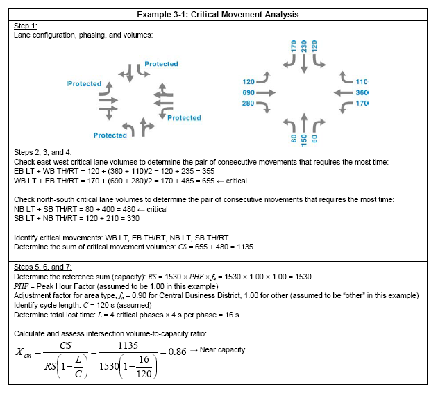
A simple example is provided in Example 3-1 to illustrate the basic elements of the procedure.
Application
From a signal timing perspective, the volume-to-capacity ratio is an important measure that defines how well progression can be achieved. For coordinated through movements, a volume-to-capacity ratio approaching capacity means that virtually all vehicles departing on green will be departing from a queue at the saturation flow rate. This type of operation is efficient in terms of maximizing the throughput of an intersection, but it greatly limits the ability to have vehicles arrive and depart on green without stopping (a typically desirable objective of progression). Therefore, if one desires to minimize stops for through vehicles along an arterial, the volume-to-capacity ratio for through movements must be kept sufficiently low (this has not be documented, but it is likely to be around 0.85 or lower) to allow a portion of the through movement’s green time to remain undersaturated. If overall volume levels are too high to permit a large enough undersaturated period for the coordinated through movements to pass through without stopping, the objective of progression through the intersection without stopping may be infeasible.
Limitations
The critical movement analysis procedure is simple and cannot accommodate all real-world conditions encountered when developing signal timing. These include vehicle and pedestrian minimum times (as noted above), assumed constant values of capacity for each lane, and complex signal phasing. For these conditions, more advanced analysis methods are likely to be more accurate. However, the critical movement analysis procedure is still often a good first approximation.
Figure 3-5 Graphical summary of Critical Movement Analysis/Quick Estimation Method (1)
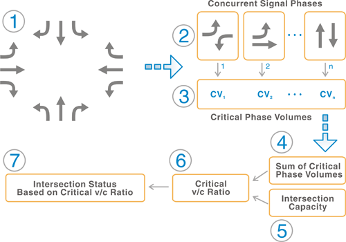
| Step | Process |
|---|---|
| 1 | Identify movements to be served and assign hourly traffic volumes per lane. This is the only site-specific data that must be provided. The hourly traffic volumes are usually adjusted to represent the peak 15-minute period. The number of lanes must be known to compute the hourly volumes per lane. |
| 2 | Arrange the movements into a desired sequence of phases that can be run concurrently based on the design of the signal. This is based in part on the treatment of each left turn (protected, permissive, etc.). |
| 3 | Determine the critical volume per lane that must be accommodated during each interval. This step determines which movements are critical. The critical movement volume determines the amount of time that must be assigned to the phase on each signal cycle. |
| 4 | Sum the critical phase volumes to determine the overall critical volume that must be accommodated by the intersection. This is a simple mathematical step that produces an estimate of how much traffic the intersection needs to accommodate. |
| 5 | Determine the maximum critical volume that the intersection can accommodate: This represents the overall intersection capacity. The HCM QEM suggests 1,530 vphpl for most purposes |
| 6 | Determine the critical volume-to-capacity ratio, which is computed by dividing the overall critical volume by the overall intersection capacity, after adjusting the intersection capacity to account for time lost due to starting and stopping traffic on each cycle. The lost time will be a function of the cycle length and the number of protected left turns. |
| 7 | Determine the intersection status from the critical volume-to-capacity ratio. The status thresholds are given in Table 3-2. |
| Critical Volume-to-Capacity Ratio | Assessment |
|---|---|
| < 0.85 | Intersection is operating under capacity. Excessive delays are not experienced. |
| 0.85–0.95 | Intersection is operating near its capacity. Higher delays may be expected, but continuously increasing queues should not occur. |
| 0.95–1.00 | Unstable flow results in a wide range of delay. Intersection improvements will be required soon to avoid excessive delays. |
| > 1.00 | The demand exceeds the available capacity of the intersection. Excessive delays and queuing are anticipated. |
Source: (2)
3.4 INTERSECTION-LEVEL PERFORMANCE MEASURES AND ANALYSIS TECHNIQUES
The capacity measures discussed above are essential for determining the sufficiency of the intersection to accommodate existing or projected demand. However, capacity by itself is not easily perceived by the user. This section presents the most common user-perceived operational performance measures and analysis techniques used in timing individual intersections.
3.4.1 Performance Measures
The two primary user-perceived performance measures used to evaluate the performance of individual intersections are delays and queues.
Control Delay and Intersection Level of Service
Delay is defined in HCM 2000 as “the additional travel time experienced by a driver, passenger, or pedestrian.” Delay can be divided into a number of components, with total delay and control delay being of most interest for signal timing purposes.
The total delay experienced by a road user can be defined as the difference between the travel time actually experienced and the reference travel time that would result in the absence of traffic control, changes in speed due to geometric conditions, any incidents, and the interaction with any other road users (adapted from the HCM definition). Control delay is the portion of delay that is attributable to the control device (the signal, its assignment of right-of-way, and the timing used to transition right-of-way in a safe manner) plus the time decelerating to a queue, waiting in queue, and accelerating from a queue. For typical through movements at a signalized intersection, total delay and control delay are the same in the absence of any incidents.
Chapter 16 of the HCM provides equations for calculating control delay; primary contributing factors are lane group volume, lane group capacity, cycle length, and effective green time. The HCM control delay equation also includes factors that account for elements such as pretimed versus actuated control, the effect of upstream metering, and oversaturated conditions. Control delay is calculated separately for each movement; intersection control delay consists of an average across all movements, weighted by volume. The HCM defines Level of Service for signalized intersections in terms of control delay using delay thresholds given in Table 3-3.
| LOS | Control Delay per Vehicle (seconds per vehicle) |
|---|---|
| A | ≤ 10 |
| B | > 10-20 |
| C | > 20-35 |
| D | > 35-55 |
| E | > 55-80 |
| F | > 80 |
| Source: (2) | |
Queue Length
Queue length is a measurement of the physical space vehicles will occupy while waiting to proceed through an intersection. It is commonly used to assess the amount of storage required for turn lanes and to determine whether the vehicles from one intersection will physically spill over into an adjacent intersection. Several queue length estimations are commonly used with signalized intersections. Average queue and 95th-percentile queue are commonly estimated for the time period for which the signal is red. However, it is sometimes useful to include the queue formation that occurs during green while the front of the queue is discharging and vehicles are arriving at the back of queue. Queues measured in this way are often noted as average back of queue or some percentile of back of queue. Appendix G to chapter 16 of the HCM 2000 provides procedures for calculating back of queue.
3.4.2 Evaluation Techniques: The HCM Procedure for Signalized Intersections
To calculate the user-based performance measures described above, the critical movement analysis procedures described previously are insufficient. The most commonly used procedure for estimating intersection-level performance measures is provided by the HCM operational analysis methodology for signalized intersections (Chapter 16 of the HCM)
Capabilities
The HCM procedure addresses many of the limitations of critical movement analysis, including the assumption of constant values of capacity for each lane and the ability to analyze different types of signal phasing. In addition, some software packages implement procedures that are adequate for many signal timing applications, even though they may or may not be exact replications of the HCM procedure
Known Limitations
Known limitations of the HCM analysis procedures for signalized intersections exist under the following conditions (adapted from 1)
- Available software products that perform HCM analyses generally do not accommodate intersections with more than four approaches;
- The analysis may not be appropriate for alternative intersection designs;
- The effect of queues that exceed the available storage bay length is not treated in sufficient detail, nor is the backup of queues that block a stop line during a portion of the green time;
- Driveways located within the influence area of signalized intersections are not recognized;
- The effect of arterial progression in coordinated systems is recognized, but only in terms of a coarse approximation;
- Heterogeneous effects on individual lanes within multilane lane groups (e.g., downstream taper, freeway on-ramp, driveways) are not recognized; and
- The procedure accounts for right turns on red by reducing the right-turn volume without regard to when the turns can actually be made within the signal cycle.
If any of these conditions exist, it may be necessary to proceed to arterial models or to simulation discussed in the next section to obtain a more accurate analysis
3.4.3 Practical Operational Approximations
In many cases, a variety of practical approximations can be used at varying stages in signal timing development. Some practitioners often rely primarily on these practical approximations and then observe and fine-tune their implementation in the field. In all cases, these practical approximations are often simple enough to be calculated in one’s head, thus providing a method ready to be used in the field or as a quick check on calculations done using more advanced techniques
Cycle length
At a planning level, it is common to assume a cycle length for a given intersection to estimate its capacity performance. If the cycle length for an intersection is unknown, common planning-level assumptions for cycle length based on the complexity of the intersection are given in Table 3-4. These assumptions do not account for cycle length requirements for coordinated operation (see Chapter 6), nor do they account for the ability for actuated intersections to vary the effective cycle length from cycle to cycle. These approximations, however, are useful in the procedures for estimating approximate queue lengths and for identifying whether a movement is substantially under or over capacity
| Signal Complexity | Commonly Assumed Cycle Length(s) |
|---|---|
| Permissive left turns on both streets | 60 |
| Protected left-turns, protected-permissive left turns, or split phasing on one street | 90 |
| Protected left-turns, protected-permissive left turn phasing, and / or split phasing on both streets | 120 |
If an analysis is to be completed for an intersection in an existing coordinated system, the user should use the current cycle length. Choosing a different cycle length would require changing the coordinated plan for adjacent intersections and could have implications throughout the system
Average and 95th-Percentile Green Time
Green time for individual movements can be approximated in many cases through estimating the number of vehicles per lane expected to be served in a given cycle and then setting an appropriate green time to serve that amount of traffic. This technique is useful for estimating green times for minor movements for which queue clearance is the primary objective and there is no intention to hold green time for vehicles to arrive and depart on green as one might do for coordinated through movements. For movements also serving pedestrians (e.g., minor-street through movements), this technique can provide an estimate of green time needed for cycles in which no pedestrian calls are placed, but it does not account for the additional time that may be required to provide pedestrian walk and clearance time
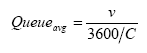
The process for estimating the average queue length for each cycle is given in Equation 3-4. It makes the simplifying and conservative assumption that the movement is timed so that all arriving vehicles for the movement arrive on red and that there is no residual queue at the end of the green. This assumption is realistic if the green time for the movement is a small percentage of the cycle length (e.g., less than 10 to 15 percent of the cycle) and thus would not apply to particularly high-volume movements.
Equation 3-4
Equation 3-5
A useful approximation for saturation flow rate is to assume a value of 1800 vehicles per hour for each lane, which results in a numerically simple value of 2 seconds of green time per vehicle. It is also useful to assume a startup lost time of approximately 2 seconds. Therefore, a queue of 4 vehicles can be assumed to take 2 + (4 × 2) = 10 seconds to clear.
One may use a Poisson distribution to estimate 95th-percentile queue from the average queue. In practice, the 95th-percentile queue is approximately 1.6 times the average queue for high-volume movements to approximately 2.0 times the average queue for low-volume movements. The following practical and simplifying approximation is useful in many cases for the purposes of signal timing, recognizing that it is overly conservative in some cases.
Equation 3-6
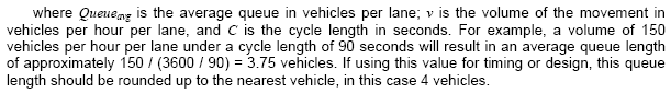
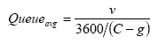
Using the example in the previous paragraph, a movement with an average queue length of 3.75 vehicles has a 95th-percentile queue length of approximately 7.5 vehicles, rounded up for timing or design purposes to 8 vehicles. This movement would need a 95th-percentile green time of 2 + (8 × 2) = 18 seconds. Some practitioners use the 95th-percentile queue for estimating green time for protected left turns and the average queue for estimating green time for protected-permissive left turns under the assumption that under protected-permissive operation, vehicles not served during the protected phase can be served during the permissive phase. This depends in part on the availability of gaps in the opposing through vehicle stream and thus may not be applicable in cases where the opposing through movement is approaching capacity. In these cases, a more detailed analysis is advisable. Another useful planning-level procedure used in design for estimating 95th-percentile queue length is to assume a value of 1 foot per vehicle being served during the hour. For example, a left-turn movement with a volume of 150 vehicles per hour would have a 95th-percentile queue length of approximately 150 feet. This procedure is most accurate for cycle lengths around 90 seconds. For shorter cycle lengths, the queue length should be shortened (e.g., by 10 to 20 percent for a cycle length of 60 seconds); for longer cycle lengths, the queue length should be extended (e.g., by 10 to 20 percent for a cycle length of 120 seconds). One could then use the value from this estimation method by assuming that each vehicle occupies a space of 25 feet and then using the techniques described above to estimate the 95th-percentile green time for the movement.
One must use caution using these practical approximations where queue length is critical. For example, if the queue from a left-turn lane exceeds available storage, it could block a through lane. If the blocked through lane is a critical movement, the performance of the entire intersection will be adversely affected, and field observations will not match office calculations.
3.4.4 Intersection-Level Field Measurement
Several field techniques can be used to measure some of the key intersection-level operational measures of effectiveness. The most common in practice is an intersection delay study. The FHWA/NTOC performance measures project selected delay (both recurring and non-recurring) as one of the measures to be considered for national standardization. Since non-recurring delay is the delay that occurs in the presence of an incident, recurring delay is the measure that is applied to evaluate signal timing. Some (but not all) of the more commonly used performance measures can be calculated from each of these techniques. These and others are described in more detail in the ITE Manual of Transportation Engineering Studies (3) and other references. This section discusses some of the more commonly used methods
Stopped Delay
A common intersection delay study is the method to estimate stopped delay. This procedure surveys a specified movement over a period of time. There are two data points collected during the survey, the total volume and the number of stopped vehicles at a given time interval. The aggregate sum of the stopped vehicles at the time interval is divided by the total entering volume to determine an average stopped delay. This method has been superseded in the HCM by the method to estimate control delay, described in the next section
Control Delay
Control delay can be measured in the field by recording the arrival and departure time of vehicles for a movement or approach. This procedure is described in detail in the HCM in Appendix A of Chapter 16. A detailed description of the methodology and a worksheet are provided. This method does not directly capture all of the deceleration and acceleration associated with control delay but is indicated in the HCM to yield a reasonable estimate of control delay. Queue formation during oversaturated conditions can make it difficult to use this method, as queues often extend beyond the measurement area and can spill into other intersections, confounding any measurements. In these cases, travel time estimates for selected origin-destination pairs (as described in the following section) may be more useful
Delay Weighting for Specific User Types
Delays can be focused primarily on vehicular traffic or can be weighted by particular vehicle types. To improve freight mobility, data collection could weight trucks more heavily than other traffic. Person delay is sometimes used by weighting the person carrying capacity of the vehicle. In these cases, transit vehicle capacity is calculated into the overall delay on the system
3.5 ARTERIAL- AND NETWORK-LEVEL PERFORMANCE MEASURES AND PREDICTION TECHNIQUES
When considering signal timing among a series of signalized intersections, as for coordinated signal operation, performance measures and models that account for the relative interaction of adjacent intersections become important. This section presents the most common performance measures, prediction techniques, and field measurements used for evaluating signal timing performance along arterial streets and coordinated networks. The measures and methodologies in this section, along with the measures for individual intersections described previously in this chapter, support the signal timing policies, the coordination techniques, and the signal timing process presented in Chapters 2, 6, and 7, respectively.
3.5.1 Arterial- and Network-Level Performance Measures
In addition to the estimation of intersection-level performance measures at each intersection along an arterial or within a network, a number of performance measures are used to assess how well the intersections fit together in terms of signal timing. These include stops, travel speed, and bandwidth and are described below. Other arterial- and network-level measures of effectiveness, including transit level of service, bicycle level of service, and pedestrian level of service, are sometimes used in developing and evaluating the effectiveness of signal timing. These are outside the scope of this document but are provided in the HCM
Stops
Stops are also used frequently to measure signal system effectiveness. Although this measure has not been identified as a candidate for standardization nationally, it is very important for two reasons:
- Stops have a higher impact on emissions than delay does because an accelerating vehicle emits more pollutants and uses more fuel than an idling vehicle. In other words, an idling vehicle must idle for many minutes before it emits as many pollutants as those emitted for a single stop.
- Stops are a measure of the quality of progression along an arterial. Motorists are often frustrated when they have to make multiple stops. In some of the signal timing software, the user is given the option of defining the relative importance of stops and delays through the use of weighting factors. If stops are assigned a high level of importance, progression on arterials will be improved, even though this may result in higher overall delay.
Motor vehicle stops can often play a larger role than delay in the perception of the effectiveness of a signal timing plan along an arterial street or a network. Stops tend to be used more frequently in arterial applications where progression between intersections (and thus reduction of stops) is a desired objective. Many software packages, including signal timing optimization programs and simulation packages, include estimates of stops.
Travel Time, Travel Speed, and Arterial Level of Service
Travel time and travel speed is one of the most popular measures used to assess how well arterial traffic progresses. Travel speed accounts for both the delay at intersections and the travel time between intersections. The HCM can be used to determine arterial level of service (LOS) based on travel speed. The HCM defines arterial LOS as a function of the class of arterial under study and the travel speed along the arterial. This speed is based on intersection spacing, the running time between intersections, and the control delay to through vehicles at each signalized intersection. Because arterial level of service is calculated using delay for through vehicles regardless of origin or destination, the resulting speed estimates may not necessarily correspond to speed measurements made from end-to-end travel time runs that measure a small subset of the possible origin-destination combinations along an arterial. Table 3-5 presents the HCM’s definitions of classes of arterials based on design and functional categories, and 0 presents the threshold speeds for each class of arterial. Further detail can be found in Chapters 10 and 15 in the HCM. Note that these level of service thresholds only reflect the perspective of vehicular travel time; they do not account for the effects on transit, bicycles, and pedestrians. A broader, multimodal perspective on arterial level of service is being considered for the next edition of the HCM.
| Functional Category | ||
|---|---|---|
| Design Category | Principal Arterial | Minor Arterial |
| High-Speed | I | N/A |
| Suburban | II | II |
| Immediate | II | III or IV |
| Urban | III or IV | IV |
| Source: (2) | ||
| Urban Street Class | I | II | III | IV |
|---|---|---|---|---|
| Range of free-flow speeds (FFS) | 55 to 45 mph | 45 to 35 mph | 35 to 30 mph | 35 to 25 mph |
| Typical FFS | 50 mph | 40 mph | 35 mph | 30 mph |
| LOS | Average Travel Speed (mph) | |||
| A | > 42 | > 35 | > 30 | > 25 |
| B | > 34-42 | > 28-35 | > 24-30 | > 19-25 |
| C | > 27-34 | > 22-28 | > 18-24 | > 13-19 |
| D | > 21-27 | > 17-22 | > 14-18 | > 9-13 |
| E | > 16-21 | > 13-17 | > 10-14 | > 7-9 |
| F | ≤ 16 | ≤ 13 | ≤ 10 | ≤ 7 |
| Source: (2) | ||||
Bandwidth, Bandwidth Efficiency, and Bandwidth Attainability
Bandwidth, along with its associated measures of efficiency and attainability, are measures that are sometimes used to assess the effectiveness of a coordinated signal timing plan. Unlike the preceding measures, bandwidth is purely a function of the signal timing plan as it is oriented in time and space; the effect of traffic is not explicitly accounted for in the calculation. As a result, bandwidth is not directly tied to actual traffic performance, although it is sometimes used as a surrogate for potential traffic performance. The use of bandwidth in developing coordinated signal timing plans is described in more detail in Chapter 6. Bandwidth is defined as the maximum amount of green time for a designated movement as it passes through a corridor. It can be defined in terms of two consecutive intersections (sometimes referred to as link bandwidth) or in terms of an entire arterial (sometimes referred to as arterial bandwidth). Bandwidth is typically measured in seconds. Two related bandwidth measures, bandwidth efficiency and bandwidth attainability, are sometimes used to normalize bandwidth measures. Bandwidth efficiency is a measure that normalizes bandwidth against the cycle length for the arterial under study. The specific formula is given in Equation 3-6
Equation 3-7
| Efficiency Range | PASSER II Assessment |
|---|---|
| 0.00 - 0.12 | Poor progression. |
| 0.13 - 0.24 | Fair progression. |
| 0.25 - 0.36 | Good progression. |
| 0.37 - 1.00 | Great progression. |
| Source: (4) | |
Bandwidth attainability is a measure of how well the bandwidth makes use of the available green time for the coordinated movements at the most critical intersection in the corridor. It is given in Equation 3-7 as follows:
Equation 3-7
Attainability, as with efficiency, is typically reported as a unitless decimal or percentage. The software program PASSER II provides guidelines to determine the quality of a particular attainability; these are given in Table 3-8. An attainability of 100 percent suggests that all available green time through the most constrained intersection is being used by the green band.
| Attainability Range | PASSER II Guidance |
|---|---|
| 1.00 - 0.99 | Increase minimum through phase. |
| 0.99 - 0.70 | Fine-tuning needed. |
| 0.69 - 0.00 | Major changes needed. |
| Source: (4) | |
Bandwidth is highly dependent on the demands on the non-coordinated phases (actuated intersections) and the offsets along the arterial. Bandwidth importance also varies based on traveler origin and destinations along a coordinated corridor. The more vehicles traveling the length of a coordinated corridor, without making turning movements, the more important bandwidth becomes as a measurement tool, and vice versa. In addition, bandwidth, travel time, and stops are related to one another; a large bandwidth will result in shorter travel times and less stops to vehicles traveling the length of the corridor
Emissions
Emissions are an important measure because they directly affect air quality. Emissions may be particularly important in the case of programs funded by Congestion Mitigation and Air Quality (CMAQ) funds, which (as the name implies) use funds allocated with the objective of improved air quality. Emissions can be estimated by some of the software packages in use
Fuel Consumption
Improved fuel efficiency of the transportation system is an important measure for reducing the costs to consumers and use of this energy source. Fuel consumption can be estimated by some of the software packages in use
Performance Index
Some software packages allow several measures of effectiveness to be mathematically combined into a single performance index, or PI. This allows an optimization routine within the software package to search for combinations of cycle lengths, offsets, and splits that achieve an optimal value of the performance index. The performance index itself is unlikely to be observable in the field, although its component measures may be observable.
3.5.2 Evaluation Techniques
Measures of effectiveness can be measured directly in the field or estimated using an analysis tool. Table 3-9 indicates the variety of field data collection and analytical techniques that can be used
| Measure | Primary Evaluation Technique | Supplemental Technique |
|---|---|---|
| Delays | Deterministic traffic analysis tool | Floating car runs (through movement or intersection observation) |
| Stops | Field data collection using manual observers or floating car runs (See text on the next page) | Floating car runs or simulation |
| Emissions | Microscopic traffic simulation | Environmental or planning models |
| Fuel Efficiency | Microscopic traffic simulation | Environmental or planning models |
| Travel Time | Floating car runs | Microscopic traffic simulation |
Arterial and Network Signal Timing Models
For many practitioners, arterial and network signal timing models are the models of choice when developing signal timing plans, particularly for coordinated systems. Arterial and network signal timing models are distinguished from the isolated intersection methods described previously by the way they account for the arrival and departure of vehicles from one intersection to the next. Traffic progression is treated explicitly through using time-space diagrams or platoon progression techniques. Some models deterministically estimate the effect of actuated parameters for both vehicles and pedestrians, typically by using a combination of scaling factors for vehicle demand and the presence or absence of vehicle and/or pedestrian calls.
A key feature of arterial and network signal timing models is the explicit effort to “optimize” signal timing to achieve a particular policy (see Chapter 2). To accomplish this, each model uses some type of algorithm to test a variety of combinations of cycle length, splits, and offsets to achieve a calculated value of one or more performance indices and then attempt to find an optimal value for those performance indices. In addition, most arterial and network signal timing models use elements of the HCM procedures to estimate certain parameters, such as saturation flow rate.
Arterial and network signal timing models are frequently the most advanced type of model needed for most signal timing applications. However, because the models described in this section are deterministic, they lose validity in cases where demand exceeds capacity or where the queues from one intersection interact with the operation of an adjacent intersection. Therefore, cases with closely spaced intersections or with intersections exceeding capacity may not be well served by these types of deterministic models. In these cases, it may be necessary to use microscopic simulation models to obtain more realistic assessments of these effects.
Microscopic Simulation Models
In the context of signal timing, microscopic simulation models can be thought of as an advanced evaluation tool of a proposed signal timing plan. Most simulation models do not have any inherent signal timing optimization algorithms and instead depend on other programs to provide a fully specified signal timing plan for evaluation. However, simulation models typically can directly evaluate the effects of interactions between intersections or the effects of oversaturated conditions or demand starvation caused by upstream oversaturated conditions. Simulation models can also be useful to estimate the effects of short lanes where either the queue in the lane affects the operation of an adjacent lane or where the queue in the adjacent lane prevents volume from reaching the subject lane.
Recent advances in technology have allowed direct linkages between simulation models and either actual signal controllers or software emulations of those controllers, known as hardware-in-the-loop (HITL) and software-in-the-loop (SITL), respectively. These in-the-loop simulations allow actual controllers and/or their algorithms to replace the approximation used in simulation models to more accurately reflect how a controller will operate. The simulation model is used to generate traffic flows and send vehicle and pedestrian calls to one or more controllers based on a detection design implemented in the simulation. The controller receives the calls as if it was operating in the field and uses its own internal algorithms to set signal indications based on the calls received and the implemented signal timing. The signal displays are passed back to the simulation model, to which traffic responds.
When running simulation analyses to compare alternatives, care is needed to ensure that the resolution of the model is sufficient to model the type of control anticipated. A simulation model, for example, typically requires precision on the order of a tenth of a second to accurately replicate gap detection. Therefore, the use of coarser resolution settings to speed up simulation run time may yield incorrect results
3.5.3 Arterial and Network Field Measurement Techniques
Data collection of arterial and network measures of effectiveness can be conducted either manually or using automated techniques. The following sections discuss some of the more commonly employed techniques in more detail
Travel Time Runs
Travel time studies evaluate the quality of traffic movements along an arterial and determine the locations, types, and extent of traffic delays. Common measures extracted from travel time runs include overall travel time, delay for through vehicles at individual intersections, number of stops, and the variability of delays and/or stops at intersections. The latter measure is often useful in demonstrating a change between uncoordinated and coordinated operation.
The floating car method is the most commonly employed technique used for travel time runs. The vehicle driver is instructed to “float” with the traffic stream, which is defined as traveling at a speed that is representative of the other vehicles on the roadway. This is accomplished by passing as many vehicles as pass the floating car (within reasonable safety limits). The floating car data is then reduced to determine the number of stops, delay time, and travel time over the route traversed by the vehicle. This process must be repeated several times to obtain good representative data.
A variety of techniques have been used to collect travel time runs, ranging from manual measurements with stop watches to more advanced techniques using portable Global Positioning System (GPS) devices. GPS output provides the vehicle’s location (latitude and longitude) and velocity. The probe vehicle begins traveling along the corridor with the GPS set to record position and speed for each second of travel. The vehicle location and instantaneous velocity allows for an estimate of the performance measures of delay, percent runs stopped, and travel time. Special inputs can also be coded to denote an event such as the location of a stop bar or bus stop, or when a parking maneuver occurs
Of the variety of performance measures that can be used to evaluate arterial performance, four can be determined by travel time runs:
- Travel Time is the total elapsed time spent driving a specific distance. The average travel time represents an average of the runs for a particular link or for the entire corridor.
- Delay is the elapsed time spent driving in a stopped or near-stopped condition, often defined as speeds less than 5 mph. The average delay represents an average of the runs for a particular intersection or for the entire corridor.
- Percent Runs Stopped is the percentage of the total number of travel time runs conducted during which a vehicle stops.
- Average Speed is the average distance a vehicle travels within a measured amount of time (this is affected by the amount of time experienced in delay).
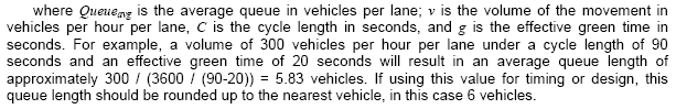
A sample travel time graph is shown in Figure 3-6 where distance along the corridor is represented along the x-axis and performance measures are plotted along the y-axis. This type of graphical display allows for ready comparison of before and after data along the corridor.
A critical factor in the success of a travel time study using vehicle probes is the skill level of the driver(s) involved. Inexperienced personnel may suddenly realize they are no longer traveling as part of the platoon and may adversely affect the platoon by inducing braking reactions in response to lane changes. This is more likely to occur in flows at or near capacity
Figure 3-6 Sample travel time run result graph
Figure 3-6 is a sample travel time graph where distance along the corridor represented x-axis and performance measures of speed delay are plotted y-axis. The plot shows impact signal timing change by contrasting before after measures. This type graphical display allows for ready comparison data corridor.
Automated Collection of Measures of Effectiveness
It is ideal to use a traffic signal system for automated collection of performance measures, but few agencies currently have that capability. In many cases, vehicle detectors are used to perform two different types of functions
The first function is to provide inputs for actuated signal control. When detectors are used for this purpose, they are typically installed near the intersection on the approaches under actuated control, which makes them less effective for performance measurements.
The second function is to act as system sensors. These detectors are typically installed at a mid-block location, which provides accurate measures of vehicle volumes and speeds. The information provided by system sensors can be used to support the following system functions:
- acquiring traffic flow information to compute signal timing
- identifying critical intersection control (CIC)
- selecting timing plans
- developing on-line and off-line timing plans through optimization programs.
Thus, the local intersection detectors are used directly by actuated controllers, whereas the system sensors are used to support the functions of the central computer or arterial master (5)
To acquire data, the loop detector is best suited to computerized traffic signal control because it is reliable, accurate, and able to detect both presence and passage. Using the presence and passage outputs, a number of variables, such as volume, occupancy, speed, delay, stops, queue lengths and travel time, can be defined to a varying degree of accuracy. These variables are related to either traffic flow along the length of the detectorized roadway or in the immediate vicinity of the detectors (5). Some of these measures of effectiveness that can be collected through loop detectors are described below.
- Volume is the quantity that is most easy to obtain. This quantity is the number of pulses measured during a given period.
- Occupancy is the percent of time that a detector indicates a vehicle is present over a total time period. Occupancy can range from zero to 100 percent, depending on vehicle spacing. Volume and occupancy are the most important variables for use in selecting traffic responsive timing plans and for many operating thresholds. In some cases, volume can be used without occupancy. It generally follows that occupancies of over 25 percent are a reliable indicator of the onset of congestion. (5)
- Speed is another useful variable used for on-line or offline computation of signal timing plans using optimization programs. For a single inductive loop detector, speed is inversely proportional to occupancy at a fixed volume. Two loops (dual loop detectors—also known as speed traps) provide much more accurate speed measurements.
3.6 SAFETY ASSESSMENT
The safety performance of signal timing is often implicitly considered but seldom explicitly evaluated. The transportation profession is in the process of developing increasingly quantitative safety methodologies to allow analysis of safety measures of effectiveness comparable to their operational counterparts. The forthcoming Highway Safety Manual (6) represents a major step in this direction. In addition, further discussion on safety analysis as applied to signalized intersections may be found in FHWA’s Signalized Intersections: Informational Guide (1); the content in this section is largely adapted from that document
Statistical techniques for evaluating collision performance vary from basic to complex. They may compare the safety performance of a single signalized intersection to another group of similar intersections, or they may serve as a screening tool for sifting through a large group of sites and determining which site has the most promise for improvement. This section provides information about safety analyses focusing exclusively on whether or not there are safety issues at an intersection that will respond to signal timing; it also provides quantitative information about estimated safety impacts of signal timing changes.
There are many factors in addition to signal timing that contribute to the safety performance of an intersection. There are also many new tools being developed to support quantitative safety analyses. Therefore, in the situation where it has been determined an intersection may respond to safety improvements, the analyst should be sure to consider more than signal timing changes as a possibility for improving safety
Crash data is of widely varying quality. In general, the less severe the collision, the less likely it is for a crash to be reported to the local jurisdiction. As a result, it is common to experience systematic underreporting of property damage only (PDO) crashes. Crashes are sometimes reported inaccurately or subsequently inaccurately entered into the database, making it difficult for the analyst to accurately identify factors contributing to crashes. It is also notable that the number of crashes that occur at a given location will vary from year to year partially due to changes in traffic volumes, weather conditions, travel patterns, and surrounding land uses, and partially due to regression to the mean. Regression to the mean is caused by the tendency for crashes at a location to fluctuate up and down over time as the average number of crashes per year converges to a long-term average. Therefore, the observed number of crashes in any given year may actually be higher or lower then the long-term average for the site.
The evaluation of crash frequency, crash patterns, and crash severity remains an important part of a safety analysis. The analyst should obtain three to five years of crash data; summarize the crashes by type, severity, and environmental collisions; and prepare a collision diagram of the crashes to help identify trends. A site visit can also be helpful in identifying causal factors. It is also possible to statistically determine if any of the crashes by type, severity, or other environmental conditions (e.g. weather, pavement, time of day) are over-represented as compared to other comparable facilities. A variety of tests and other evaluative tools are discussed further in FHWA’s Signalized Intersections: Informational Guide (1)
3.6.2 Quantitative Safety Assessment
Signal timing is one of many factors which may contribute to crashes. Other factors may be horizontal and vertical alignment conditions, roadside features, sight distance, driver compliance with traffic control, access management near intersections, driver expectations, and roadway maintenance and lighting. If the purpose of the project is to update intersection signal timing, the analyst should be aware of the potential impacts to safety. Alternatively, if the site has been identified as one needing safety improvements the analyst should be aware that signal timing is one of many possible countermeasures for improving safety at an intersection. Table 3-10 provides a summary of crash types and possible signal timing changes to benefit safety.
| Collision with Another Vehicle | Single-Vehicle Collision | |||||||||
|---|---|---|---|---|---|---|---|---|---|---|
| Signal Timing Change | Angle | Head-On | Rear-End | Sideswipe—Same Direction | Sideswipe—Opposite Direction | Collision with Bicycle | Collision with Parking Vehicle | Collision with Pedestrian | Overturned | Run Off Road |
| Provide left-turn signal phasing | x | x | x | x | x | |||||
| Optimize clearance intervals | x | x | ||||||||
| Restrict or eliminate turning maneuvers (including right turns on reds) | x | x | x | x | x | x | ||||
| Employ signal coordination | x | x | x | |||||||
| Implement emergency vehicle pre-emption | x | x | x | x | x | x | x | x | ||
| Improve traffic control of pedestrians and bicycles | x | x | x | |||||||
| Remove unwarranted signal | x | x | x | |||||||
| Provide/improve left-turn lane channelization* | x | x | x | x | x | |||||
| Provide/improve right turn lane channelization* | x | x | x | x | x | |||||
* While not technically part of signal timing, these have a significant impact on safety and should be considered. See the FHWA Signalized Intersections: Informational Guide (1) for more information. Ref: 9, Appendix 10
Accident modification factors (AMFs) are used as a way to quantify crash reductions associated with safety improvements. These factors are developed based on rigorous before-after statistical analysis techniques that account for, among many factors, regression to the mean, sample size, and the effects of other treatments from the estimation process. AMFs which have been calculated using reliable before-after analyses will be quantified and will often also include a confidence interval. AMFs below 1.0 will likely have a safety benefit, and AMFs greater than 1.0 may degrade safety conditions. For example, studies have found that converting a 4-legged urban intersection from stop control to signal control will have an AMF for all fatal and injury crashes of 0.77. This means that there will be an anticipated reduction in crashes of 23 percent if a traffic signal were installed
Quantitative AMFs can be found in many sources (7, 8, 9). The most reliable sources are those that estimate AMFs using the more sophisticated before-after analytical techniques. In the future, the Highway Safety Manual (6) and the final report for NCHRP 17-25 “Crash Reduction Factors for Traffic Engineering and ITS Improvements” will also contain numerous AMFs. In addition, local jurisdictions can also develop their own AMFs based on studies conducted locally.
3.7 SIGNAL WARRANTS
Warrants for signalization are intended to create a minimum condition for which signalization may be the most appropriate treatment. Each of the warrants is based on simple volume, delay, or crash experience at the location before signalization is installed. None accounts for the specific design of the signal or the way it may be timed (e.g., pre-timed versus actuated). As a result, an engineering evaluation should be conducted in conjunction with the evaluation of signal warrants to determine that the proposed signalization plan actually represents an improvement over existing conditions.
The eight warrants presented in Chapter 4C of the 2003 MUTCD are as follows (10)
- Warrant 1, Eight-Hour Vehicular Volume. This warrant consists of two volume-based conditions, Minimum Vehicular Volume and Interruption of Continuous Traffic, of which one or both must be met over an eight-hour period.
- Warrant 2, Four-Hour Vehicular Volume. This warrant is similar to Warrant 1 but relies on volume conditions over a four-hour period.
- Warrant 3, Peak Hour. This warrant is primarily based on delay to minor movements during peak hour conditions.
- Warrant 4, Pedestrian Volume. This warrant is intended for conditions where delay to pedestrians attempting to cross a street is excessive due to heavy traffic on that street. It consists of minimum pedestrian volumes and available gaps in traffic.
- Warrant 5, School Crossing. This warrant is similar to Warrant 4 except that it is specifically intended for school crossing locations.
- Warrant 6, Coordinated Signal System. This warrant is intended to allow signals that may assist in progression of traffic. It is only intended for use where the resulting signal spacing is not less than 1,000 feet (300 m).
- Warrant 7, Crash Experience. This is the only specific safety-related warrant and is satisfied by a frequency of crashes over a specific period of time that can be corrected through the use of signalization.
- Warrant 8, Roadway Network. This warrant may be used to support the use of a signal to concentrate traffic at specific locations.
As noted in the MUTCD, “the satisfaction of a traffic signal warrant or warrants shall not in itself require the installation of a traffic control signal” (Section 4C.01, 10).
Signalization is not always the most appropriate form of traffic control for an intersection, and it is sometimes possible to create a larger benefit by removing a traffic signal than by retiming it
The MUTCD acknowledges this by stating that “since vehicular delay and the frequency of some types of crashes are sometimes greater under traffic signal control than under STOP sign control, consideration should be given to providing alternatives to traffic control signals even if one or more of the signal warrants has been satisfied.” (10). Potential alternatives include the use of warning signs, flashing beacons, geometric modifications, and/or conversion of the intersection to a stop-controlled intersection or a roundabout.
3.8 REFERENCES
- Rodegerdts, L., B. Nevers, B. Robinson, J. Ringert, P. Koonce, J. Bansen, T. Nguyen, J. McGill, D. Stewart, J. Suggett, T. Neuman, N. Antonucci, K. Hardy, and K. Courage. Signalized Intersections: Informational Guide. Report No. FHWA-HRT-04-091. Federal Highway Administration, Washington, D.C., August 2004.
- Transportation Research Board. Highway Capacity Manual 2000. National Academy of Sciences, Transportation Research Board, Washington, D.C., 2000.
- Institute of Transportation Engineers. Manual of Transportation Engineering Studies. H. D. Roberson, ed. Institute of Transportation Engineers, Washington, D.C., 2000.
- Wallace, C. E., E.C.P. Chang, C. J. Messer, and K. G. Courage, "Methodology for Optimizing Signal Timing (M¦O¦S¦T), Volume 3: PASSER II-90 Users Guide," prepared for the Federal Highway Administration, COURAGE AND WALLACE, Gainesville, FL, December 1991.
- Traffic Detector Handbook, 2nd ed. Report No. FHWA-IP-90-002. Federal Highway Administration, Washington, D.C., July 1990.
- Transportation Research Board. Highway Safety Manual. Anticipated publication 2009.
- National Cooperative Highway Research Program (NCHRP). NCHRP Research Results Digest 299. Washington, DC: Transportation Research Board of the National Academies, November 2005.
- Elvik, R. and T. Vaa. The Handbook of Road Safety Measures. Amsterdam: Elsevier Ltd., 2004.
- Antonucci, N.D., Hardy, K.K., Slack, K. L., Pfefer, R., and Neuman, T. R., “NCHRP Report 500 Volume 12: A Guide for Addressing Collisions at Signalized Intersections.” Washington, D.C., Transportation Research Board, National Research Council, 2004.
- Federal Highway Administration. Manual on Uniform Traffic Control Devices. Washington, DC: Federal Highway Administration, 2003.