Comprehensive Truck Size and Weight Limits Study - Modal Shift Comparative Analysis Technical Report
Appendix F: Rail Financial Model
The process for estimating the post-diversion impact on the rail industry that could result from the decreased number of rail shipments and rate reductions to hold onto traffic is described in this appendix. The objective of this analysis is to compute a revised rail industry balance sheet, for the analysis year 2011 for the illustrative 2014 CTSW Study scenarios. In this way, the scenario impact on revenue, freight service expense (FSE), contribution, and ROI resulting from changes in traffic can be assessed.
The rail impact analysis employs two models, the US Department of Transportation's Intermodal Transportation and Inventory Cost (ITIC) Model and an Integrated Financial Model described in Figure F-1. Both are discussed below. These models required inputs from: 1) Class I railroad financial and operating statistics as compiled by the Association of American Railroads (AAR) in the Analysis of Class I Railroads-2011; and 2) the 2011 Surface Transportation Board's (STB's) Carload Waybill Sample. The data used from the Analysis of Class I Railroads is compiled from R-1 reports submitted by the railroads to the STB.
The revenue and traffic diversions used to assess rail impacts are derived from the ITIC Model. The model uses the STB Carload Waybill Sample as the basis for rail freight flows and estimates transportation and inventory costs for moving freight by rail and truck under different truck size and weight (TSW) scenarios.
In this analysis, the ITIC model allows the railroads to respond to increased truck competition by lowering their own rates down to variable cost, if necessary, to prevent diversion of rail freight to trucks. If motor carriers can offer shippers lower transportation and inventory costs than rail variable cost plus inventory costs, then the model assumes that the railroad will lose the traffic and it will divert to truck. As truck transportation costs decrease, the rail industry will experience three separate but related post-diversion effects:
- Fewer rail shipments will reduce rail revenue.
- As the railroads offer discounted rail rates to shippers to compete with motor carriers, additional revenue will be lost.
- As rail ton-miles decrease due to losses in traffic, the unit (ton- mile) costs of handling the remaining freight traffic will increase.
It is important to note that for diverted traffic, railroads lose revenue and some costs. When discounting to hold traffic, railroads lose revenue but all costs remain.
The post-diversion effects listed above are measured by the following key ITIC model outputs: 1) the remaining rail revenues after accounting for losses in revenues from both diversion and from discounting to hold traffic, and 2) the remaining post-diversion ton-miles used to assess the effect of diversion on rail FSE.
The ITIC Model provides values for revenue and ton-miles for both the base case and each scenario. Percent changes from the base case to the scenario were calculated from these values. These percent changes were then applied to financial and operating statistics collected by the AAR to determine the revenues and ton-miles used as inputs into an Integrated Financial Model.
The Integrated Financial Model was used to estimate the impact that changes in TSW regulations would have on the rail industry's financial condition. This is the same model used to estimate financial impacts on the railroads for the 2000 CTSW Study. As inputs, this model uses ITIC model outputs and the change in FSE with respect to changing ton-miles (cost elasticity) derived in the STB's Christensen study, "A Study of Competition in the U.S. Freight Railroad Industry and Analysis of Proposals that Might Enhance Competition (Volume 2, p. 9-11)." The methodology for applying the elasticity was best described by Gerard McCullough in his 1993 dissertation, A Synthetic Translog Cost Function for Estimating Output-Specific Railroad Marginal Costs. The FSE represents variable cost, the variable and fixed cost portions of depreciation charges, and interest expense railroads' incur.
According to Christensen Associates more recent measure, the cost elasticity for the industry is 0.862. As railroads lose traffic, measured in ton-miles, and the associated revenues, reductions in cost do not decrease in a one-to-one relationship with ton-miles as noted by the elasticity value, 0.862. Rather, railroads shed costs much more slowly because of the high fixed and common cost component of total costs that characterize the industry. To illustrate, if there were a 10 percent decline in rail ton-miles, the application of the 0.862 elasticity coefficient indicates that freight cost would decline only 8.6 percent. As a consequence, the cost to handle the remaining traffic in terms of cost per ton-mile would increase in the post-diversion case as would be expected in a decreasing cost industry. This increased cost for remaining rail traffic represents an offset to shipper cost savings experienced by truck and former rail shippers as a result of truck size and weight changes, yielding the net national change in shipper costs.
Figure F-1 presents a "wiring diagram" that demonstrates how the Integrated Financial Model works. The model links the Income Statement, Sources and Uses of Funds, and Balance Sheet information, as well as ROI for the rail industry, to evaluate each of the truck size and weight scenarios under consideration. The model imports the independent variables noted above -percent changes in revenues and ton-miles - from the ITIC model into the Income Statement to calculate the effects on the industry balance sheet. By using measured changes in the Income Statement variables-revenues, expenses (including FSE), income, and cash generated and expended-the model produces a revised industry Balance Sheet as output. The output includes a new FSE resulting from a change in ton-miles. The Integrated Financial Model is also used to calculate the post-diversion ROI, and the increase in rail rates that would be required to return the rail industry to pre-diversion financial conditions.
Figure F-1 Integrated Financial Model of the Railroad Industry
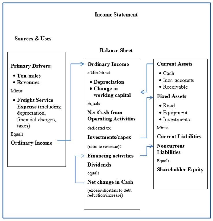
The following is an explanation of the Integrated Financial Model.
What is an Integrated Financial model?
In order to evaluate the financial outcomes, the team used the Vanness Brackenridge Group Economic and Financial Model. This model is fully integrated from source data to analytical sectors to economic-financial reports. The model structure is comprehensive in that it provides reports at various levels of reporting detail. This model has been used in many assignments worldwide.
An integrated model assessment (sometimes called enterprise modeling) links the Income Statement, Sources and Uses of Funds, and Balance Sheet information as well as Rate of Return (IRR) or Net Present Value (NPV) of the enterprise evaluated, for the scenarios under consideration. This allows the user to declare or import independent variables for activity and financial drivers, under various scenarios, for the choices under study.
MODEL STRUCTURE
|
Overall Reporting Sectors: |
Supporting Report Sectors (as req'd): |
|---|---|
|
Activity levels Statement of Revenues Statement of Expenses Income Statement Cash Flow Statement Investment/Debt Portfolio Balance Sheet Capital Investment Schedule(s) |
Activity levels by type/distance Tariffs by type/distance/other fares Staffing and productivity Material and supply requirements Fuel consumption module reporting by type Public Service Obligation (Subsidy) module Capital Program by specific elements Equipment utilization and rents |
Income Statement Primary Drivers:
Among the primary independent variables that have been specified are:
- Ton-Miles
- Revenues
- Freight Service Expenses
- Depreciation
- Fixed Charges
- Income Taxes.
Sources and Uses of Funds (Cash Flow) Significant Assumptions:
- Income from Continuing Operations Depreciation and Amortization is carried from the Income Statement.
- Increase/Decrease in Deferred Taxes.
- Increase/Decrease in Accounts Receivable and other Current Assets Increase/Decrease in Accounts Payable and Other Current Liabilities
- Investments/Capital
- Dividends Principal Payments on Debt/Finance Leases
- All Other Accounts
Balance Sheet Significant Assumptions:
- Current Assets Gross Fixed Assets (Road, Equipment, etc.) before depreciation
- Accumulated Depreciation and Amortization
- Current Liabilities Total Non-Current Liabilities, the sum of long term debts, lease liabilities and deferred tax credits.
- Shareholders' Equity is the sum of Current and Net Fixed Assets minus Current and Non-Current Liabilities.
Discussion of Increased Costs of Handling Post Diversion Traffic and "Contribution Effects"
Post diversion, the rail industry and the individual railroads will suffer on two counts. They will lose the revenue associated with the diverted movements. But they will also suffer increased marginal costs to move the traffic which remains.
This increased cost to move the remaining traffic reduces any beneficial effects on total logistics costs (in "systemic" terms) from truck diversion at lower apparent cost and cuts against railroad profitability as well.
The Financial Model has been programmed to calculate new operating costs for reduced ton-miles of activity and including the effect of increasing marginal cost as a result of volume loss.
Calculating Post Diversion Costs
Calculation of post diversion operating cost equivalents is a two-step process. Christensen Associates have given us the elasticity of modified Freight Service Expenses (FSE) with respect to changing ton-miles which for the industry as a whole is 0.862.
First, a new FSE is estimated, based on the changed ton-miles post diversion. The higher cost level, due to decreasing efficiencies of scale, is calculated and compared with the cost level prevailing at the base case level of activity. As a practical matter of calculation, the formulas are conveniently expressed in terms of the aggregate cost levels, and then compared as follows;
Step 1. Predicted FSE (Cost) change for given level of ton-miles change:
x * e * C1 = C2
Where: x = percent change in ton-miles; e = coefficient of change in FSE (cost) relative to a change in ton-miles ; C1 = base FSE; C2 = new FSE post-diversion;
Step 2. The second step in this process entails computing the change in cost levels attributable to the loss of volume, and, therefore, the increased marginal cost for handling remaining post diversion railroad traffic.
Base case cost per ton-mile:
C1/Q1 = CCM1 Where: CCM1 = base case cost per ton-mile
Post diversion ton-miles traveling at the old CCM1 cost per ton-mile:
((Q1(1-x)) * CCM1 = C3 Where C3 = Q2 volume moved at old cost per ton-mile
And, comparing C2 with C3 yields the increased costs attributable to higher post diversion marginal cost per ton-mile:
C2 - C3= Increased cost to handle post diversion ton-miles.
or C3 = (e-1)*C1*x
Discussion of the Concepts of Diversion Impacts on Rail Industry Finances
Revenue Loss:
An analysis of financial impact of diversions on the industry must take into effect both revenue and cost components. Revenue losses will result from the out of hand losses due to the diversion of traffic per se. A "second order" effect would be the predictable rail response to the losses, namely the temptation to cut competing rates. The diversion model takes this into account by hypothetically lowering rail rates on competing traffic to the variable cost threshold, but not beyond. Both revenue elements are provided to the economic and financial model. The latter rate decreases could be claimed as a net benefit, were it not for the following phenomenon.
A "third order" and more subtle effect derives from the temptation of the railroads to raise rates for other traffic to replace the revenues lost. In effect, the railroads could be predicted to try to replace the lost contribution from any given level of revenues lost. Their options for doing so would, however, be limited. Ultimately, only captive shippers[34] could be tapped for additional revenues. Non-captive shippers might pay increased rates temporarily, but would eventually bolt, leading to another round of diversions, losses and retaliation. Thus, all but captive should be ruled out as a long term source of make-up revenues, were it possible to precisely define who is and who is not a captive shipper. Unfortunately, that is not within the scope of this 2014 CTSW Study, so here it is assumed remaining rail shipments are at least "short term captive" within the time frame of the 2014 CTSW Study.
[34] Generally, captive shippers are those which do not enjoy viable competitive alternatives to the serving rail carrier by virtue of the product shipped or their location or both. return to Footnote 34
previous | next