3. Framework for Economic Analysis
Standard approaches to highway benefit-cost analysis do not include the full stream of benefits specific to freight carriage (e.g., benefits stemming from business reorganization effects). A standard analysis of a highway investment takes account of benefits to immediate highway users: time savings, reduction in operating costs, and reduction in accident costs. Benefits from savings in truck travel time are calculated with an estimate of the average wage of the drivers. In the context of freight benefits, these are benefits to the owner of the truck (the carrier), but they do not include benefits to the owner of cargo (the shipper).
Costs of truck operation do not, however, provide a sufficient means of estimating the value of time in freight carriage; the impact on the shipper must be included as well. In industries with relatively high logistics costs, the greater share of gains from freight improvement may well go to the shipper rather than the carrier. Time-cost reductions—reductions in transit time and increases in reliability—have substantial value for shippers. These values need to be estimated and added to the benefits treated in the standard analysis in a manner that appropriately deals with potential double counting issues.
But that is, by no means, the whole story of bringing freight into the benefit-cost framework. There are significant effects of freight improvements beyond the immediate cost reductions for carriers and shippers. Improvements in the freight-movement system may allow companies to change their modes of operation in ways that lead to further gains in productivity. In a paper written over thirty years ago, Herbert Mohring and Harold Williamson referred to this as the "reorganization effect." Improved transportation may let firms realize economies of density or scale, for example, by building bigger plants, warehouses, or stores, because a single facility can serve, or draw supplies from, a larger area owing to better transportation.
Much of a firm's response to transportation-cost reduction will be reorganization of its logistics. It will respond to the lower costs by moving goods longer distances, using fewer warehouses, and carrying less inventory for a given level of sales. It will buy more transportation and realize gains from improved logistics. But firms can make other changes in the ways they do things; lower costs might lead to product improvements, for example. We need to be clear about the different kinds of effects that may flow from freight-transportation improvement; they have to be treated differently in the analysis. The following classification scheme is helpful.
| First-order Benefits | Immediate cost reductions to carriers and shippers, including gains to shippers from reduced transit times[2] and increased reliability. |
|---|---|
| Second-order Benefits | Reorganization-effect gains from improvements in logistics[3]. Quantity of firms' outputs changes; quality of output does not change. |
| Third-order Benefits | Gains from additional reorganization effects such as improved products, new products, or some other change. |
| Other Effects | Effects that are not considered as benefits according to the strict rules of benefit-cost analysis, but may still be of considerable interest to policy-makers. These could include, among other things, increases in regional employment or increases in rate of growth of regional income. |
The first part of the Freight BCA Study is concerned with the first and second-order benefits of improved freight transportation. At this stage, we are, thus, concerned with immediate cost reductions, including time-cost reductions for shippers, and with reorganization-effect improvements in logistics. The challenge is to bring the first and second-order benefits together in such a way that they are fully counted, but nothing is counted twice.
In the first-order case, nothing changes for shippers except the cost of freight movement (including time cost). They continue to ship the same volume of goods the same distance between the same points. Their costs are less, but they make no response to the cost reduction other than to keep the extra income thus realized. In order to estimate the first-order benefits, it is necessary to find the value of the time-cost reductions and then add this amount to those that are calculated in a standard analysis—reductions in operating costs, cost savings from reductions in accidents, and drivers' wages—all assuming no change in volumes or distances shipped.
In the second-order case, firms respond to the cost reduction. They may reduce prices to gain additional revenue by selling more goods; they may ship longer distances; they may close some warehouses; they may do some combinations of these things; or they may do something else altogether. The first-order case, taken by itself, is an unrealistic scenario. In the real world, a firm would make some kind of response to any noticeable cost reduction. We make the conceptual separation between the first and second-order cases because it helps us follow the path of causality and because it helps us fit these phenomena into the economic concepts of supply and demand. Cost reductions of a certain magnitude occur; firms respond in ways that lead to both greater output and lower cost per unit of output.
We look at demand for freight carriage from the viewpoint of the consumer of freight transportation, i.e., the shipper. A shipper's response to the change in freight-movement cost is determined by the conditions of its demand for freight transportation. A shipper's demand for freight transportation reflects both the market's demand for the firm's products and the way in which it uses freight transportation as an input to its production and/or distribution processes.
The conditions of demand are embedded in a curve or equation called a "demand curve." In our context, the curve shows the amount of freight transportation a firm will buy at various levels of freight cost, including time costs. The demand curve in Exhibit 4 takes two forms, D0 and D1. D0 shows the firm's demand for freight transportation before the improvement takes place. The new curve, D1, shows the change in demand that follows the improvement. But the change in demand is not immediate; it reflects a firm's response to the cost reduction, a response that will occur over some considerable period of time.
Recall that a shipper's demand for freight transportation reflects both the market's demand for the firm's products and the way it uses freight transportation as an input. The market demand for the products is not affected by the freight improvement, nor, at the first instance, is the way the firm uses freight transportation. The way a shipper uses freight transportation refers to its basic logistical arrangements, especially number and location of warehouses. The shipper's reaction to the cost reduction can be thought of as occurring in three phases, as illustrated in Exhibit 3.
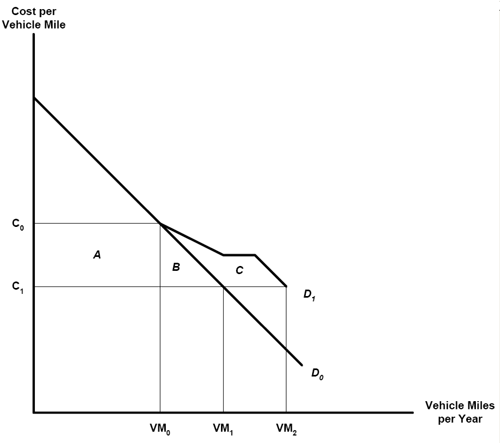
Exhibit 3: Demand Curve for Transportation
Exhibit 3 shows the cost reduction from C0 to C1 on the vertical axis. In the very short run, the shipper makes no response and continues to buy the same number of vehicle miles of freight, VM0. The benefit to the shipper is the area A, the cost reduction with the existing volume of freight. In the next phase of response, the shipper takes advantage of the lower cost and buys more freight movement, VM1. This adds the area B to the benefit. But this still reflects the shipper's original demand curve, D0. The shipper has not made any changes in the firm's basic logistical arrangements.
But, after managers have had time to consider the cost reduction, they may, as already noted, make changes in their basic logistical arrangements. This is when the shipper's demand for transportation would change, and there would be the new freight-transportation demand curve, D1. The additional benefit from the reorganization is area C, the area between the old and new demand curves. The freight improvement's full benefit is reflected in the sum of areas A, B, and C. This captures all benefits with no double counting.
The meaning of the shift in the demand curve requires some additional explanation. The shipper's demand curve reflects the benefits the shipper gets from buying freight transportation. The cost the shipper is willing to incur to obtain freight transportation is what managers believe the freight movement is worth to the firm. They will not incur a cost higher than what they think it is worth (although they will willingly take it at a lower cost if that is possible). Thus, the change in the demand curve reflects the greater benefits the shipper can get from the freight-carriage improvement, once the firm has reorganized its logistics set-up.
An important extension of this point is that the full benefit to the shipper is also the full benefit to society, as defined by the strict canons of benefit-cost analysis.[4] This is because consumers' demand for the shipper's product is embedded in the shipper's demand for inputs, including freight transportation. If, for example, the shipper makes gizmos, the social benefits from gizmo consumption are reflected in the shipper's demand for all the inputs necessary to make gizmos.[5] Whatever benefits are realized by gizmo consumers are captured in the gains to the shipper, as measured by the combination of the reduction in costs (area A) and the increase in the shipper's consumer surplus (areas B and C).[6] (Please note that what is being measured here is not the increase in the shipper's profits. That is something different.)
Note that most of the discussion here is in terms of one firm buying freight carriage. The economic concepts set out here will apply with equal validity to many firms—all the firms, for example, affected by a freight-transportation improvement. We have developed a sound conceptual framework for the Freight BCA. We need a method for estimating the actual values that go with these theoretical constructs.
- Carrier effects include reduced vehicle operating times and reduced costs through optimal routing and fleet configuration. Transit times may affect shipper in-transit costs such as for spoilage, and scheduling costs such as for inter-modal transfer delays and port clearance. These effects are non-linear and may vary by commodity and mode of transport.
- Improvements include rationalized inventory, stock location, network, and service levels for shippers.
- All the benefits we are considering under the first and second-order cases count as social benefits by the strictest rules, providing there is no double counting. As the classification of effects in Exhibit 3 shows, there are a number of effects that may be of interest to citizens and to decision makers but are not benefits to society as reckoned by economic theory. As the table shows, such effects might include regional redistribution of income, regional employment effects, impacts on land values, or other effects. These effects might be shifts of benefits from one group to another, or they might be other reflections of the benefits already counted in the strict framework. In technical economic language, the benefits in A+B+C account for all the benefits to society from the freight improvement. This point is demonstrated mathematically in a paper by Herbert Mohring and Harold Williamson, published in 1969. That paper and the argument it presents are discussed in technical terms in the White Paper on the analytical framework that accompanies this paper.
- When we refer to "social benefits" here, it should be understood that we refer to the gross benefits of the freight improvement without subtracting costs to arrive at a net figure. Our underlying theoretical argument says there are no external benefits, all benefits are captured in the shippers' demand curves. When, in a later stage, we address costs, we will definitely find external costs that have to be added to the calculation.
- The economic concept of consumers' surplus reflects the fact that the total amount consumers pay for a particular good or service is less than what that good or service is actually worth to them. Different people will place a different value on a good. But, generally speaking, sellers are unable to discriminate among buyers according to their different values. The price prevailing in a market reflects the value placed on a good by that consumer (or consumers) who, among those who are buying, places the least value on that good, the "marginal consumer." Others buying would be willing to pay more. For these consumers, there is a surplus, the difference between the price they pay and the actual value to them. See Appendix A for more on consumers' surplus.