| Skip
to content |
|
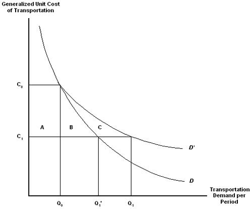
2. User Manual2.1 Version HistoryThis User Manual refers to release 1, version 2.5 of the Highway Freight Logistics Reorganization Benefits Estimation Tool. It was developed by HDR Decision Economics under the direction of the U.S. Department of Transportation, Federal Highway Administration, Office of Freight Management and Operations. 2.2 Tool PurposeThe Highway Freight Logistics Reorganization Benefits Estimation Tool estimates total benefits associated with highway investment by establishing a relationship between elasticity of demand with respect to highway performance, elasticity of demand with respect to price, a set of other region-specific variables, and the conventionally measured freight benefits resulting from travel time savings and other user benefits. The purpose of this manual is to provide users with step-by-step instructions on using the Benefit Estimation Tool, describe the data inputs required, and provide background on the sources and uses of the "default" data provided in the model. The outputs resulting from the Benefit Estimation tool indicate the additional benefit related to reorganizing logistics that may be expected to occur following from a planned performance improvement. These benefit outputs may be used in (or added to) BCAs that do not independently account for the value of improved freight management. 2.3 Additive Freight Benefit Economic Framework and Calculation Approach2.3.1 Microeconomic FrameworkFigure 2 shows the microeconomic framework that identifies the benefits of industrial reorganization. Area A represents the immediate benefits of a highway improvement to existing highway users (mainly user time savings and reduced vehicle operating costs). Area B represents the immediate benefits accruing to users newly attracted to the highway by virtue of the improvement. Areas A and B represent the benefits conventionally measured in a CBA. Area C represents the value of efficiency gains to the economy due to industrial reorganization precipitated by the highway improvement. Industrial reorganization means the adoption of advanced logistics for a firm depends on the likelihood of a threshold level of reliability in highway performance. Defined as the ratio of area C to the sum of areas A and B (C/[A+B] expressed as a percentage), the "additive freight reorganization benefit" gives the percentage by which to increase the value of conventionally-measured benefits to freight traffic in order to approximate total benefits – that is, benefits inclusive of the reorganization effect.
To assess the quantitative significance of the additive reorganization benefit, the Additive Freight Benefit Calculation considers:
Using national highway performance data, Phase II of the FHWA Benefit Cost Study found that variable-elasticity in the form of the present and post-reorganization demand curves (indicating constant returns to scale) provides a reasonable description of the available data. Specifically, the elasticity of demand for transport with respect to generalized cost is found to vary proportionately with generalized cost. The elasticity is smaller when generalized cost is relatively low and higher when generalized cost is relatively high. This implies that demand is more sensitive to changes in highway conditions when congestion is high than when congestion is low. The form of the estimated demand curve is:
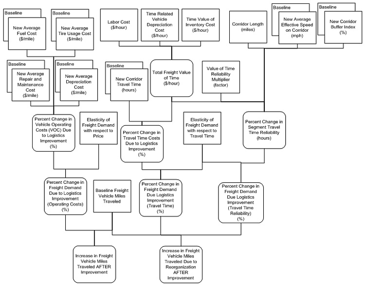
where Q is the quantity of transportation that would be demanded at a generalized cost of C, and where 2.3.2 Additive Benefit Calculation ApproachThe additive benefit estimation tool has been developed to accommodate outcomes from consumer surplus models where the practitioner explicitly accounts for induced demand using standard transportation demand elasticity estimates and estimates the change in consumer surplus resulting from a candidate highway investment. The tool calculates the additive benefit using the logic laid out in the structure and logic diagram below.
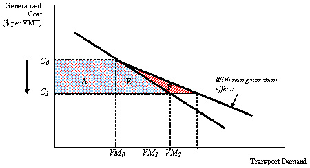
Additive Benefit Estimation with Consumer Surplus ModelsIn Figure 4, the additive benefit factor would be calculated as the ratio of area F (the area between the long run transport demand curve "with reorganization effects," the standard short-run demand curve, and the
In other words, the additive benefit factor is estimated as the percentage change in consumer surplus resulting from incremental transport demand along the long-run demand curve (incremental transport demand is illustrated by the shift from
A numerical example of additive benefit estimation with consumer surplus models is provided in Table 2.
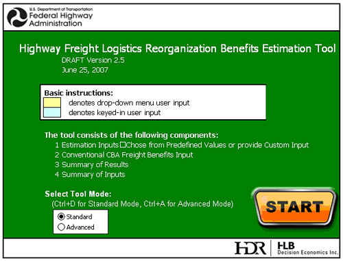
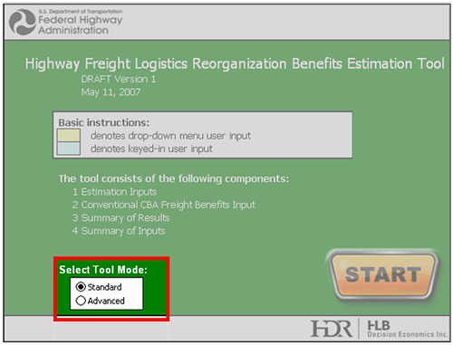
*Numbers in red signify key variables that illustrate the change in demand. 2.4 Opening ScreenThe opening screen of the Highway Freight Logistics Reorganization Benefits Estimation Tool provides the user with some basic information on the tool, such as the tool's name and version, basic user instruction, outline of the tool's components, mode selection, and start button. Figure 5 provides a screenshot of the tool's opening screen.
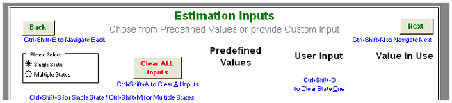
Tool Name and Version: The tool name and model version are helpful during user support inquiries. Basic Instructions: The basic instructions provide the user with an understanding of the color coding applied to user input. Light yellow cells indicate a drop-down menu is available for the user to select. Only values that are contained in the dropdown list will be accepted for input. Light blue cells indicate keyed-in user input. Users must key-in the input for these cells, although certain cells may only accept specific types of keyed-in data. Tool Composition: Provides an overview of the four main screens of the estimation tool. The user will encounter these screens in sequential order using the model navigation buttons. Tool Mode: The tool may be operated in two modes, Standard or Advanced. Standard Mode is recommended for most users. Advanced mode allows the user access to additional inputs, such as price elasticities, which should only be altered if the user has specific knowledge and understanding of these values and their impact on the estimation of benefits. Start Button: The start button will take the user to the first of the four main model screens, "Estimation Inputs." Click the start button to begin estimation of freight logistic benefits. 2.5 Estimation Inputs ScreenThe Estimation Inputs Screen gathers key data from the user regarding the segment data for the specific roadway improvement being analyzed. The header at the top of the Estimation of Inputs Screen contains key navigation and option items for the screen, as well as headings to identify each column. When a state or states are selected, predefined values will populate for all of the key inputs. For specific information, sources and descriptions of the estimation inputs refer to the data dictionary appendix. A screenshot of this header is shown in Figure 6.
Navigation ButtonsAt each corner of the screen, there are green navigation buttons. The Back button can be used to navigate back to the Opening Screen and the Next button can be used to navigate forward to the following screen in the tool. State Mode SelectionThe tool is configured to handle one or two states. In the event that a project segment is entirely contained within one state, the Single State option button should be selected. In the event that the project segment crosses a state border, and the project encompasses two states, the Multiple State option button may be selected. Selecting the Multiple State option button will expand the screen to handle two states, and users will be required to input certain values for each state, such as value of time or vehicle mix. Clear ButtonsThe Clear All Inputs button will clear all user inputs on the Estimation Inputs screen. When the Multiple States option is enabled, users are also able to clear inputs for a single state with the option buttons: Clear State 1 and Clear State 2 appearing under the User Input column heading. Users are prompted to confirm they wish to clear all inputs. Note: Once the inputs are cleared, they cannot be restored. Column HeadingsIn single state mode, the tool is structured to have three key input columns: Predefined Values, User Input, and Value in Use. When a state is selected, the predefined values will be populated based on research values. These predefined values may be state specific, national averages, or calculated based on other inputs. For specific information, sources and descriptions of the estimation inputs refer to the data dictionary appendix. The User Input column allows users to override the predefined value and input their own values for each of the inputs. The Value in Use column displays which value the tool uses in its calculations. When the User Input column is blank, the Predefined Values are used. If a User Input value is entered, it will be reflected in the Value in Use column. In the two-state mode, the three columns are duplicated to handle input for multiple states when necessary. 2.5.1 Project InformationThe first section on the Estimation Inputs screen is the Project Information section. This section gathers basic information for the project for record keeping. The information contained in this section will be included in the summary output sheets for the user's record.
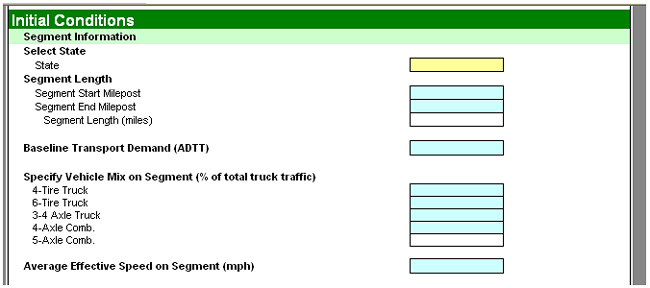
Project NameInput project name for recordkeeping purposes. OperatorInput tool operator's name for recordkeeping purposes. DateInput today's date for recordkeeping purposes. Internal Version NumberInput an internal version number for recordkeeping purposes. This will be helpful in keeping track of results if the input data is updated. 2.5.2 Initial ConditionsThe second section on the Estimation Input screen is for Initial Conditions on the segment. This section establishes the baseline for the estimation of benefits. It is composed for Segment Information, Value of Time, Vehicle Operating Costs and Reliability of Travel Time subsections. All inputs in this section should represent conditions before the planned improvement. This should represent present day information. 2.5.2.1 Segment InformationThe segment information section captures key inputs that are specific to the roadway segment being analyzed. Information such as the state in which the project is located, the segment length, baseline truck traffic, truck vehicle mix and average effective speed are collected in this section. Although the tool offers predefined values for all input data, it is strongly recommended that users input data specific to their segment, as these values vary greatly segment by segment.
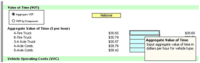
StateSelect a state from the dropdown menu. Selection of a state will population the tool with predefined values based on the state that is selected. For information on data sources and use, see Section 2.9.1.1. Segment LengthInput the start milepost and end milepost. Based on this information, the tool will calculate the segment length. The start milepost must be less than the end milepost. For information on data sources and use, see Section 2.9.1.2. Baseline Transportation Demand (ADTT)Input baseline transportation demand, in terms of ADTT. For information on data sources and use, see Section 2.9.1.3. Specify Vehicle Mix on SegmentInput the distribution of vehicle types by truck type as a percentage. This represents the share of a specific type of truck as a percentage of total truck traffic (not of total roadway traffic). These values must total to 100% for trucks on the segment. For information on data sources and use, see Section 2.9.1.4. Average Effective Speed on SegmentInput the average effective speed on the segment in miles per hour. For information on data sources and use, see Section 2.9.1.5. 2.5.2.2 Value of Time (VOT)The VOT subsection gathers baseline information about the average value of time for truck traffic along the segment. These values aggregate to dollars per hour. There are two options when inputting value of time data: aggregate or by component. The user may select the desired option by clicking on the appropriate option button. Additionally, some of the predefined inputs for VOT are available at the state level. Users have the option to select either national or state level (or two-state blend in the two-state tool version) for the predefined values. The national level should be selected if a user believes much of the traffic is from out of state, otherwise the state option should be selected. The tool will default to values based on national averages. For information on data sources and use, see Section 2.9.2. Aggregate VOTWhen the Aggregate VOT option button is selected, the user should input the total VOT, by vehicle type, in dollars per hour.
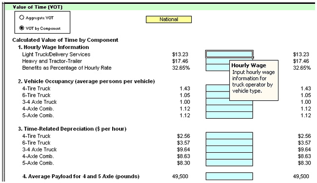
VOT by ComponentThe VOT calculation is made up of the numbered components below. Figure 10 provides a screenshot of VOT by component input area for the first four VOT components.
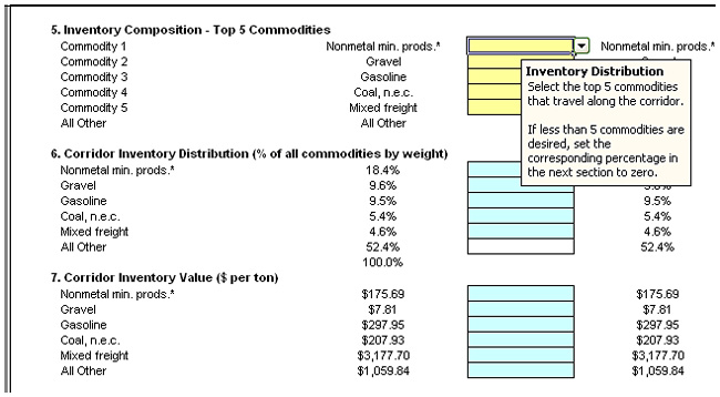
Figure 11 provides a graphical overview of the inventory component of the VOT calculation.
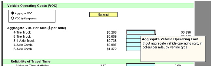
2.5.2.3 Vehicle Operating Costs (VOC)There are two options when inputting VOC data: Aggregate or by Component. The user may select the desired option by clicking on the appropriate option button. As with the VOT subsection, users have the option to select either national or state level (or two-state blend in the two-state tool version) for the predefined values. The national level should be selected if a user believes much of the traffic is from out of state, otherwise the state option should be selected. The tool will default to values based on national averages. For information on data sources and use, see Section 2.9.3. Aggregate Vehicle Operation CostsWhen the Aggregate VOC option button is selected, the user should input the total vehicle operating costs, by vehicle type, in dollars per mile.
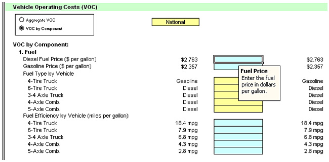
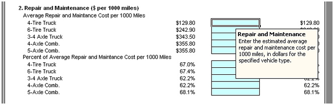
VOC by ComponentVOC is made up of the following components.
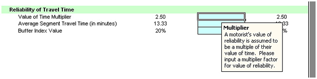
2.5.2.4 Reliability of Travel TimeReliability of Travel Time is the final, initial-state value component. This accounts for the degree of certainty around a given trip along a segment. Lower variance in travel time results in a greater degree of reliability; whereas greater variance in travel time leads to uncertainty and a low degree of reliability. Reliability of travel time is composed of three components: 1) a value of time multiplier, 2) an average segment travel time, and 3) the buffer index value. The following screenshot provides an overview of the "Reliability of Travel Time" section. For information on data sources and use, see Section 2.9.4.
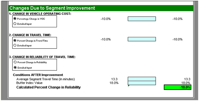
Value of Time MultiplierInput the value of time multiplier as a multiplicative factor. For information on data sources and use, see Section 2.9.4.1. Average Segment Travel TimeInput the average travel time along the segment in minutes. For information on data sources and use, see Section 2.9.4.2. Buffer Index ValueInput the buffer index value as a percentage. For information on data sources and use, see Section 2.9.4.3. 2.5.3 Changes Due to Segment ImprovementThe transportation improvement project is assumed to have a beneficial impact on freight traffic that travels along the segment. In this tool, an improvement can affect any of the three value components identified under the Initial Conditions section: 1) VOT, 2) VOC, and 3) Reliability of Travel Time. Changes can be entered as either a percentage or as specific changes to detailed input. Option buttons allow the user to select either "Percentage Change" or "Detailed Input." The format of the detailed input is similar to the input under the Initial Conditions section. 2.5.3.1 Changes Represented as a Percentage ChangeFigure 18 shows a screenshot of the Change section with all three change types represented as percentages.
In the percent change mode, the tool prompts users for inputs to three change categories:
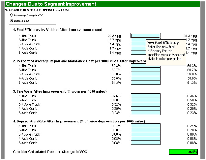
Changes in the three components should be entered as a negative number to show an improvement along the segment. For example, a negative change in VOC represents a reduction in VOC, i.e. a savings to the vehicle operator when traveling along the segment after the improvement relative to travel before the improvement. Percentage Change in VOCInput the Change in VOC represented as a percentage change over the VOC specified under the Initial Conditions section. Note: A negative value represents an improvement in VOC as this represents a decrease in the per mile vehicle operating cost. Percentage Change in Travel TimeInput change in travel time represented as a percentage change over the travel time specified under the Initial Conditions section. Note: A negative value represents an improvement in travel time and translates into a decrease in the time necessary to travel along the segment. Percentage Change in Reliability of Travel TimeInput change in reliability of travel time is represented as a percentage change over the reliability of travel time specified under the Initial Conditions section. Note: A negative value represents an improvement in reliability travel time and translates into a decrease in the uncertainty around to travel time along the segment. 2.5.3.2 Changes Represented as a Detailed InputDetailed Input Change in VOCWhen the "Detailed Input" option button under "Change in Vehicle Operating Cost" is selected, the user will be prompted to input changes to VOC by component. The changes affect the usage rate components for VOC. The value components are held constant in order to isolate the benefits caused by the segment improvement. Figure 19 provides a screenshot of the detailed input change in the VOC section.
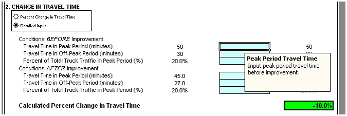
Detailed Input Change in Travel TimeWhen the "Detailed Input" option button under "Change in Travel Time" is selected, the user will be prompted to input change in travel time by detailed input. The changes affect the value of time cost across the segment. The change only impacts the travel time component, holding all other elements of value of time constant in order to isolate the benefits from the segment improvement. Figure 20 provides a screenshot of the detailed input change in travel time section.
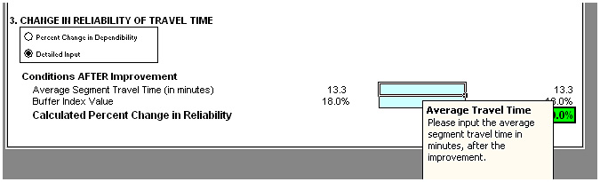
Detailed Input Change in Reliability of Travel TimeThe detailed input Change in Reliability of Travel Time section is similar to the Reliability of Travel Time input section. This section prompts users for conditions after the roadway improvement along the segment. The value of travel time and its multiplier are held constant in order to isolate the impacts of the segment improvement.
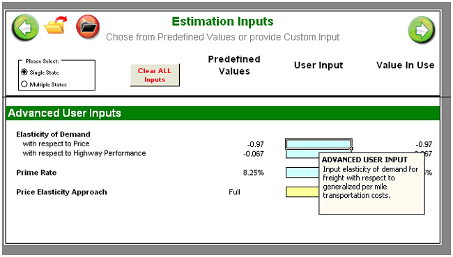
2.5.4 Advanced User InputsThis tool offers the user the option to modify some inputs that have been identified as advanced. In order to enable the Advanced User Input section, the tool mode must be set to Advanced on the Opening Screen. The screenshot in Figure 22 provides a graphical view of the Opening Screen tool mode selection.
When enabled, the Advanced User Input section is the final input section of the tool. It prompts users for inputs on elasticities of demand, interest rate, and elasticity approach. Figure 23 provides a screenshot of the Advance User Inputs section.
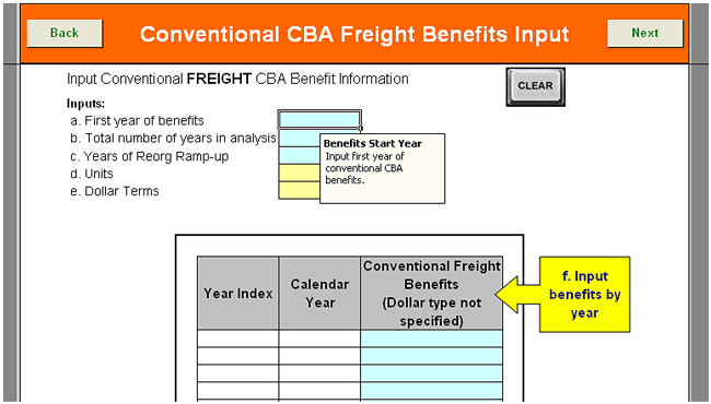
2.5.4.1 Elasticity of DemandWith Respect to PriceInput the elasticity of demand for freight with respect to price. Note: This input should only be modified if specific, accurate data exists to override the predefined value in the tool. For information on data sources and use, see Section 2.9.5. With Respect to Highway PerformanceInput the elasticity of demand for freight with respect to highway performance. Note: This input should only be modified if specific, accurate data exists to override the predefined value in the tool. For information on data sources and use, see Section 2.9.5. 2.5.4.2 Prime RateInput the prime interest rate, expressed as a percentage. Note: The prime rate is published by the Federal Reserve Bank and may be updated on a periodic basis. For information on data sources and use, see Section 2.9.5.2. 2.5.4.3 Price Elasticity ApproachSelect either the "Full" or "Additive" price elasticity approach. Note: If the user does not have specific knowledge as to the price elasticity approach, the predefined value should not be altered. For information on data sources and use, see Section 2.9.5.3. 2.6 Conventional CBA Freight Benefits Input ScreenThis screen allows for the input of freight benefits from a conventional highway CBA. These benefits would be obtained from an analysis outside this tool that was conducted for the same road segment that is currently being analyzed within this tool. Simple results may be obtained if this screen is skipped; however, it is recommended that the user complete this screen in order to obtain the full functionality of the tool. Figure 24 provides a screenshot of the header area for the "Conventional CBA Freight Benefits Input" screen. Note: Only benefits that are attributable to freight should be entered on this screen, not total highway-user benefits.
Navigation ButtonsAt each corner of the screen, there are green navigation buttons. The left button can be used to navigate back to the "Estimation Inputs" screen and the right button can be used to navigate forward to the following screen in the tool. Clear ButtonThe user may select the "Clear" button in the upper right corner of the screen to clear all inputs on this screen. A warning will prompt the user before clearing all inputs. Note: Once the inputs are cleared, they cannot be restored. Inputs:
2.7 Summary of Results ScreenThis screen requires no user input. It provides a summary of the results calculated by the tool based on user inputs from the previous two screens. Results are presented as three outcomes:
The screen header is similar to the headers in the previous screens. A screenshot of the header is provided in Figure 25.
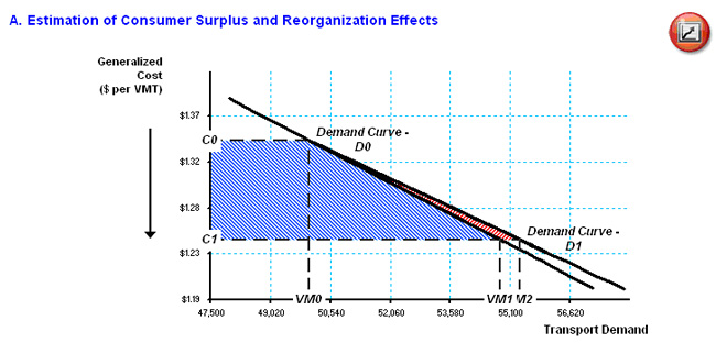
Navigation ButtonsAt each corner of the screen, there are green navigation buttons. The left button can be used to navigate back to the Conventional CBA Freight Benefits input screen, and the right button can be used to navigate forward to the following screen in the tool. Print ButtonThere is a print button to the right of the screen title. Clicking this button will bring up the print dialog box where the user can select the print options and print the results sheet. Navigation HyperlinksBelow the screen title are navigation hyperlinks that allow the user to quickly move to a specific section of the results screen. The three sections are: 1) Consumer Surplus, 2) Benefits Charts, and 3) Benefits Table. A. Estimation of Consumer Surplus and Reorganization EffectsThe first section of the Summary of Results screen provides the user with information on the estimation of demand for freight in both a graphical and tabular format. This section displays the Estimation of Consumer Surplus and Reorganization Graph. This represents the additive freight benefits that are estimated in this tool. Figure 26 provides an example of the Consumer Surplus Graph.
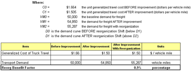
The area below the graph summarizes the key data points on the graph with their values and an explanation of what each point represents. Following this is a table that summarizes generalized travel costs, transportation demand, and the reorganization benefit factor. A screenshot example of this summary information is provided in Figure 27.
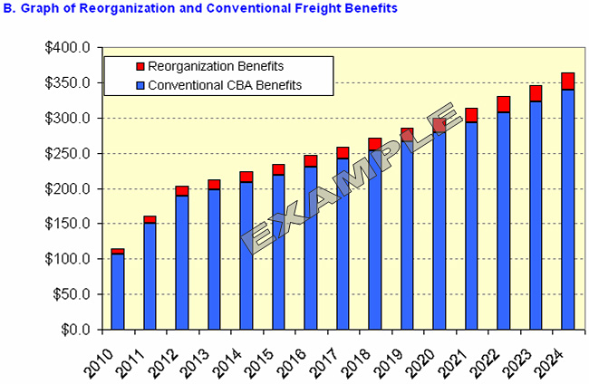
B. Estimation of Consumer Surplus and Reorganization EffectsIf conventional CBA benefits are entered on the previous screen, this section will provide a summary table of total benefits, composed of reorganization benefits and conventional CBA benefits. Figure 28 provides an example of this graph.
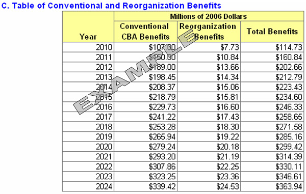
In addition to the graph, a table below the graph provides a summary of conventional CBA benefits, reorganization benefits, and total benefits (conventional + reorganization) by year. Figure 29 below provides an example of this table.
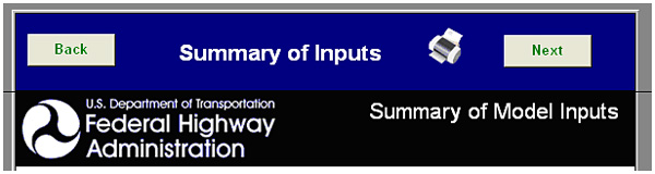
2.8 Summary of Inputs ScreenA summary of inputs screen is provided as a final screen in the tool. This screen is for summary only and requires no user input. It allows users to keep a record of the inputs used to generate the results. This is helpful if future updates for a specific project are entered into the tool. The screen header is similar to the headers in the previous screens. A screenshot of the header is provided in Figure 30.
Navigation ButtonsAt the left corner of the screen, there is green navigation button. This button can be used to navigate back to the Summary of Results input screen. On the right corner there is a red home button. This button can be used to navigate back to the tool's Opening Screen. Print ButtonThere is a print button to the right of the screen title. Clicking this button will bring up the print dialog box where the user can select the print options and print the summary of inputs sheet. This screen provides a summary of all inputs used in the model. In the single-state model, only one column is shown for the relevant state. In the two-state models, two columns are shown with state specific input for each column. In the event that inputs are entered at the segment level, for example segment length or change in VOC, these items are shown centered across both state columns. The "Summary of Inputs" screen is structured in the same format as the "Estimation Inputs" screen. The key sections are the "Initial Conditions," "Changes," and, if enabled, "Advanced Inputs." 2.9 Data DictionaryThe Data Dictionary contains information regarding the data and its uses in the calculations of the estimation tool. The tool estimates additional freight benefits in the form of generalized freight transportation costs savings due to a roadway improvement project. Generalized transportation costs are categorized into three main groups: 1) Value of Time, 2) Direct Vehicle Operating Costs, and 3) Value of Reliability. This section provides a comprehensive summary of all input data used in the model, definitions, uses, and data sources where applicable. The section provides a definition of the key input data, as well as its use in the model. Additionally, a description of the tool's predefined data and sources, where applicable, are provided. 2.9.1 Segment InformationThis section contains basic information about the highway segment being analyzed. 2.9.1.1 StateDefinition: The state in which the project is located. Use: The state selection list is used to identify the state that the project takes place in and to obtain state specific predefined data values that vary by state or region. In the event of a two-state project, the user must select the 'multiple states' option button, and specify the percentage of the project within each state. Data: List contains all 50 states in the United States and the District of Columbia. 2.9.1.2 Segment LengthDefinition: The total distance covered by the roadway segment being analyzed. This tool elicits segment length by gathering user input on start and end milepost. Use: Tool requires segment-start milepost and segment-end milepost to calculate total segment length. Data: The predefined values for segment start and end mileposts are simply placeholders for these values in the estimating tool. These are segment specific values, and it is highly recommended that users update this data with project specific values. 2.9.1.3 Baseline Transport Demand (Average Daily Truck Traffic)Definition: Average Daily Truck Traffic (ADDT) is the total number of trucks that travel on a given segment in a year, divided by 365. Use: Baseline transport demand, in ADDT, is used to calculate the baseline from which improvements are measured. Data: The predefined value for baseline transport demand is simply a placeholder for this value in the estimating tool. This is a segment specific value, and it is highly recommended that users update these data with project specific values. 2.9.1.4 Vehicle MixDefinition: Vehicle mix for truck traffic represents the average composition of truck traffic by truck type along the segment. It is the percentage of a specific truck type's roadway share relative to total truck traffic within a specific segment. Truck types, as provided by Highway Economic Requirements System (HERS), are listed below:
Use: Vehicle mix is used to determine the distribution of vehicles by type within the study corridor, which is used to assign weighting factors to key variables that are vehicle type specific. Data: The predefined values for vehicle mix is taken from the U.S. Census Bureau's 2002 Economic Census. Source: For truck types, Highway Economic Requirements System (HERS). For distribution: U.S. Census Bureau, 2002 Economic Census. Web link: http://www.census.gov/svsd/www/vius/products.html 2.9.1.5 Average Effective Speed (miles per hour)Definition: Average Effective Speed (AES) is the modified unconstrained average speed that exists for a highway section. It is the maximum speed allowed given terrain type, grade, curvature, number of heavy trucks, facility type, number of lanes, speed limit, volume-to-capacity (VC) ratio, pavement roughness, speed limit enforcement, safety concerns, and congestion, as modified by the effects of speed-changes and stop cycles (including idling time associated with these effects).[4] Use: AES is utilized to convert hourly values, such as value of time, into mileage related values. Data: The predefined values for average effect speed are simply placeholders for this value in the estimating tool. Average effective speed is highly dependent on roadway specific values. It is highly recommended that users update these data with project specific values. 2.9.2 Value of Time (VOT)The VOT calculation is composed of three main categories: labor costs, vehicle depreciation costs, and inventory timeliness cost. The calculations follow those laid out in HERS 2002. 2.9.2.1 Average Hourly WageDefinition: Average hourly wage represents the average hourly payment received by employees in the truck driver occupation. Use: A key component in the calculation of hourly value of time. Wages for the "'Truck Drivers, Light or Delivery Services" are applied to the 4-Tire Truck category, and wages for "'Truck Drivers, Heavy and Tractor-Trailer" are applied to the remaining truck categories. Data: Waged data was collected for 50 states, District of Columbia, and national level for the following occupations:
Source: U.S. Department of Labor, Bureau of Labor Statistics, Occupational Employment and Wages, May 2007. Web link: http://www.bls.gov/oes/current/oes_nat.htm 2.9.2.2 Employee Benefits as a Percentage of Hourly RateDefinition: Employee Benefits as a Percentage of Hourly Rate represents the percentage of an employee's total compensation that accounts for benefits beyond their monetary salary. Use: Utilized in the calculation of hourly value of time, in conjunction with hourly wage data. Data: National average value for employee benefits as a percentage of total compensation, for the transportation and warehousing sector. Source: U.S. Department of Labor, Bureau of Labor Statistics, National Compensation Survey, National Average for Transportation and Warehousing in 2005, Benefits as Percentage of Hourly Rate. Web link: http://www.bls.gov/ncs/ 2.9.2.3 Vehicle OccupancyDefinition: Vehicle Occupancy is the average number of people traveling in a vehicle. Use: Utilized in the calculation of hourly value of time. Data: Average vehicle occupancy, measured in average number of persons in a vehicle, by the following vehicle types:
Source: HERS-ST v2.0, Highway Economic Requirements System – State Version, Technical Report, Federal Highway Administration, U.S. Department of Transportation, 2002. 2.9.2.4 Time-Related DepreciationDefinition: Time-related depreciation is the average dollar amount that a vehicle's value declines by for each hour of use. This depreciation value is accounts for deprecation as a result of aging, independent of mileage-related deprecation (which is covered under the Vehicle Operating Costs section). Use: Utilized in the calculation of hourly value of time. Data: Average time-related vehicle depreciation, in dollars per hour, by vehicle type:
Source: U.S. Department of Transportation, Federal Highway Administration, HERS-ST v2.0, Highway Economic Requirements System – State Version, Technical Report, 2002. Web link: https://permanent.access.gpo.gov/lps57467/lps57467/isddc.dot.gov/OLPFiles/FHWA/010945.pdf 2.9.2.5 Average Payload (pounds)Definition: Average payload in pounds represents the average weight of the inventory carried in 4- and 5-axle vehicles along a highway segment. Use: It is utilized in the calculation of hourly value of time, specifically in the inventory cost component of value of time. The average payload, measured in pounds, in conjunction with other variables, is used to calculate the average payload value for 4- and 5-axle combination vehicles. Data: This is the average payload, in pounds, for 4- and 5-axle combination vehicles. In the value of time calculation, inventory costs are only calculated for 4- and 5-axle combination vehicles, in accordance with HERS guidelines. Source: U.S. Department of Transportation, Comprehensive Truck Size and Weight (CTS&W) Study, August 31, 2000. Web link: https://www.fhwa.dot.gov/reports/tswstudy/ 2.9.2.6 Inventory CompositionDefinition: Inventory composition represents the key commodities that account for a majority of the freight movement along the corridor. This tool elicits inputs for the top five commodities, by weight, on the segment, along with a catchall category for all other commodities. Use: Inventory composition is another factor in the inventory cost component calculation for value of time. It is used in conjunction with inventory value, average payload, and inventory distribution to calculate the inventory cost component of value of time. Data: Inventory composition comes from the standard commodity types utilized in FHWA's Freight Analysis Framework (FAF). Source: U.S. Department of Transportation, Federal Highway Administration, Freight Analysis Framework (FAF1 and FAF2) database, Federal Highway Administration, 2002. Web link: http://ops.fhwa.dot.gov/freight/freight_analysis/faf/index.htm 2.9.2.7 Inventory DistributionDefinition: Inventory distribution represents a commodity's share of total commodity traffic as a percentage, by weight, along the segment. Use: Inventory distribution is another factor in the inventory cost component calculation for VOT. It is used in conjunction with inventory value, average payload, and inventory composition to calculate the inventory cost component of value of time. Data: Commodity flow data (type and volume) were collected for 58 distinct corridors from the FAF database. Distribution was determined using a specific commodity's volume relative to total commodity volume within a corridor. Source: U.S. Department of Transportation, Federal Highway Administration, Freight Analysis Framework (FAF1 and FAF2) database, 2002. Web link: http://ops.fhwa.dot.gov/freight/freight_analysis/faf/index.htm 2.9.2.8 Corridor Inventory Value ($ per ton)Definition: This is the average value of commodity shipments by commodity type along a segment, in dollars per ton. Use: Inventory value is another factor in the inventory cost component calculation for value of time. It is used in conjunction with inventory distribution, average payload, and inventory composition to calculate the inventory cost component of value of time. Data: Value, tons, and ton-miles of freight shipments within the United States by domestic establishments. Source: U.S. Department of Transportation, Bureau of Transportation Statistics, and U.S. Department of Commerce, Census Bureau, 2002 Commodity Flow Survey: United States (Washington, DC: December 2004), table 5a. Table 1-53: Value, Tons, and Ton-Miles of Freight Shipments within the United States by Domestic Establishments, 2002. Web link: http://www.census.gov/svsd/www/cfsdat/2002cfs.html 2.9.3 Vehicle Operating Costs (VOC)VOC is composed of fuel costs, repair and maintenance costs, tire usage costs, and mileage related depreciation costs. VOC calculations are based on the guidelines detailed in the 2002 HERS-ST Technical Report. 2.9.3.1 Fuel CostsVehicle fuel costs are dependent on a number of factors, including fuel price, fuel type, and fuel efficiency. Fuel PriceDefinition: Fuel price ($ per gallon) is the average price per gallon for either regular unleaded fuel or for highway diesel. Use: Utilized in conjunction with fuel efficiency and fuel type to calculate the fuel cost portion of vehicle operating costs. Data: Data has been collected on the price in dollars per gallon for regular unleaded fuel and on highway diesel fuel for all 50 U.S. states, District of Columbia, and national averages. Source: U.S. Department of Energy, Energy Information Administration, U.S. Retail Gasoline and Diesel Prices. Web link: http://tonto.eia.doe.gov/dnav/pet/pet_pri_gnd_dcus_nus_w.htm Fuel Type by VehicleDefinition: This is the type of fuel, either gasoline or diesel, most commonly used by a vehicle class. Use: Utilized to assign the fuel type prices (either gasoline or diesel) to each of the five truck vehicle types. Data: Predefined values for fuel type most commonly used by each vehicle type. Options include "Gasoline," "Diesel," and "50/50 Mix" (in the event that a vehicle type may not solely use either gasoline or diesel). Fuel type is assigned for each of the HERS truck vehicle types:
Fuel Efficiency by VehicleDefinition: Fuel efficiency, measured in miles per gallon is the output in the miles traveled that a vehicle gets for one gallon of fuel consumed. Use: Utilized in conjunction with fuel prices to calculate the fuel cost portion of vehicle operating costs. Data: Data on fuel efficiency, in mpg, for each of the HERS truck vehicle types:
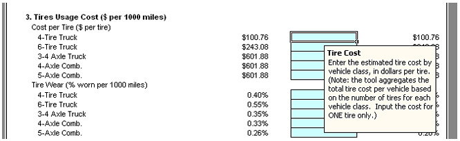
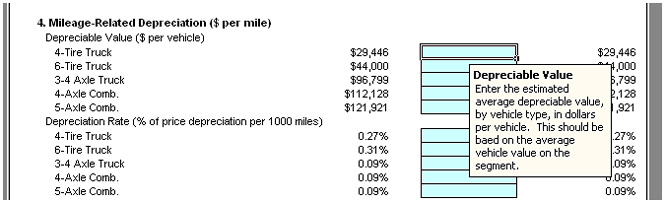
Source: Fuel efficiency based in mpg is calculated in the tool using HERS formulas, by vehicle type, based on average effective speed (all formulas assume zero grade) Web link: https://permanent.access.gpo.gov/lps57467/lps57467/isddc.dot.gov/OLPFiles/FHWA/010945.pdf 2.9.3.2 Repair and Maintenance CostsRepair and maintenance costs are composed of both a value component and a usage rate. The value component is the average repair and maintenance cost per 1,000 miles, in dollars. The usage rate is the percent of the average repair and maintenance cost per 1,000 miles used in 1,000 miles of travel in a given segment. Average Repair and Maintenance Cost per 1,000 MilesDefinition: This is the average cost per 1,000 miles for truck repair and maintenance expenses, by truck type. Use: Utilized in the repair and maintenance calculation as part of total per mile vehicle operating costs. Data: Data on average repair and maintenance cost per 1,000 miles in dollars by truck type. Source: HERS-ST v2.0, Highway Economic Requirements System – State Version, Technical Report, Federal Highway Administration, U.S. Department of Transportation, 2002. Web link: https://permanent.access.gpo.gov/lps57467/lps57467/isddc.dot.gov/OLPFiles/FHWA/010945.pdf Percent of Average Repair and Maintenance Cost per 1000 MilesDefinition: This is the percentage of the average cost per 1,000 miles for truck repair and maintenance expenses realized in travel along a given segment by truck type. Use: Utilized in the repair and maintenance calculation as part of total per mile vehicle operating costs. Data: This usage rate is calculated in the tool using HERS formulas by vehicle type based on average effective speed (all formulas assume zero grade). Source: U.S. Department of Transportation, Federal Highway Administration, HERS-ST v2.0, Highway Economic Requirements System – State Version, Technical Report, 2002. Web link: https://permanent.access.gpo.gov/lps57467/lps57467/isddc.dot.gov/OLPFiles/FHWA/010945.pdf 2.9.3.3 Tire Usage CostsTire usage costs are composed of both a value component and a usage rate. The value component is the average cost per tire, by truck type, in dollars. The usage rate is the percent of tire worn in 1,000 miles of travel on a given segment. Tire CostDefinition: This is the average cost per tire by truck type. Use: Utilized for the tire usage cost calculation as part of the total per mile vehicle operating costs. Data: Tire cost in dollars per miles by truck type. Source: U.S. Department of Transportation, Federal Highway Administration, HERS-ST v2.0, Highway Economic Requirements System – State Version, Technical Report, 2002. Web link: https://permanent.access.gpo.gov/lps57467/lps57467/isddc.dot.gov/OLPFiles/FHWA/010945.pdf Tire Wear RateDefinition: This is the percent of tire worn in 1,000 miles traveled along a given segment. Use: Utilized for the tire usage cost calculation as part of the total per mile vehicle operating costs. Data: The tire usage rate is calculated in the tool using HERS formulas, by vehicle type, based on average effective speed (all formulas assume zero grade). Source: U.S. Department of Transportation, Federal Highway Administration, HERS-ST v2.0, Highway Economic Requirements System – State Version, Technical Report, 2002. Web link: https://permanent.access.gpo.gov/lps57467/lps57467/isddc.dot.gov/OLPFiles/FHWA/010945.pdf 2.9.3.4 Mileage-Related DepreciationMileage-related depreciation costs are composed of a value component and a usage rate. The value component is the average depreciable truck value by truck type in dollars. The usage rate is the percent of the average value depreciated every 1,000 miles on a given segment. Depreciable ValueDefinition: This is the total depreciable value of a truck, by truck type. It is based on the total cost of a new truck, net of any residual value. Use: Utilized in the calculation of mileage related depreciation, which is a portion of total per mile vehicle operating costs. Data: Total depreciable value of a truck by truck type in dollars. Source: U.S. Department of Transportation, Federal Highway Administration, HERS-ST v2.0, Highway Economic Requirements System – State Version, Technical Report, 2002. Web link: https://permanent.access.gpo.gov/lps57467/lps57467/isddc.dot.gov/OLPFiles/FHWA/010945.pdf Depreciation RateDefinition: This is the rate at which a truck's depreciable value depreciates per 1,000 miles of use on a given segment. Use: Utilized in the calculation of mileage related depreciation, which is a portion of total per mile vehicle operating costs. Data: The percent of price depreciation per 1000 miles on a segment, by truck type. This usage rate is calculated in the tool using HERS formulas, by vehicle type, based on average effective speed (all formulas assume zero grade). Source: U.S. Department of Transportation, Federal Highway Administration, HERS-ST v2.0, Highway Economic Requirements System – State Version, Technical Report, 2002. Web link: https://permanent.access.gpo.gov/lps57467/lps57467/isddc.dot.gov/OLPFiles/FHWA/010945.pdf 2.9.4 Value of Reliability ($/hr-sd)The value of reliability is a proxy for the cost of uncertainty in travel time. The greater the variability in travel time, the higher the cost to the driver. When there is more certainty in travel time, the cost falls since drivers do not have to budget as much time to ensure timely delivery when traveling on a given segment. It is composed of a value component, the average travel time, and the buffer index, which captures uncertainty around travel time. 2.9.4.1 Value of Time MultiplierDefinition: This is the factor by which truck drivers value their time with respect to variability in travel time. It is applied to the value of time. Use: Utilized in the calculation of the value of reliability, to assign the value component. Data: This is a multiplier for the value of time. It uses the defined value of time in the tool by truck type to determine the value of reliability. Source: NCHRP Report 431, "Valuation of Travel-Time Savings and Predictability in Congested Conditions for Highway User-Cost Estimation," 1999. Web link: http://www.trb.org/TRBNet/ProjectDisplay.asp?ProjectID=496 2.9.4.2 Average Segment Travel TimeDefinition: This is average amount of time it takes to travel along a given segment. Use: Utilized in the calculation of the value of reliability as a baseline for the application of the buffer index percentage. Data: The predefined value is calculated using the average effective speed and the segment length, which are inputs to the tool. Source: Calculated within the tool. 2.9.4.3 Buffer Index ValueDefinition: This is the extra time buffer needed to ensure on-time arrival for most trips along a given segment. Use: Utilized in the calculation of the value of reliability to determine the amount of uncertainty around travel time. Data: The predefined value is calculated using the average effective speed and the segment length, both inputs to the tool. Source: Texas Transportation Institute, Monitoring Urban Freeways in 2003: Current Conditions and Trends from Archived Operations Data, December 2004. Web link: http://mobility.tamu.edu/mmp/FHWA-HOP-05-018/findings.stm 2.9.5 Advanced User Inputs2.9.5.1 Elasticity of DemandElasticity of Demand with Respect to PriceDefinition: This variable represents the change in demand for freight due to a change in the price of freight where the price of freight is represented by the direct vehicle operating costs. An elasticity of -0.97 means that a 10% increase in the price of freight will result in a 9.7% decrease in the demand for freight. Use: This value is used to calculate the change in freight demand due to a change of the price of freight. When vehicle operating costs fall due to an improvement in freight logistics, this elasticity value is used to calculate the impact on freight demand. Data: The predefined value is based on findings in the source report. Source: HLB Decision Economics, Meta-Analysis of Logistics Cost and Transport Demand in Relation to Freight Transportation, Draft Report, July 2001. Elasticity of Demand with Respect to Highway PerformanceDefinition: This variable represents the change in demand for freight due to the change in delay. For example, with an elasticity of -0.0076, with other things being equal, a 10% increase in delay per mile reduces freight demand by 0.076%. Use: This value is used in the calculation of changes in freight demand due to changes in travel time and the reliability of travel time in the estimation tool. Data: This value was calculated as part of the source analysis for three regions in the United States, using statistical regression techniques where demand for daily truck traffic is specified as a function of delay and real per capita income growth. Source: U.S. Department of Transportation, Federal Highway Administration, Office of Freight Management and Operations, Analysis of Regional Benefits of Highway-Freight Improvements, Draft Final Report. Prepared by HLB Decision Economics Inc., in association with ICF Consulting, June 2006. 2.9.5.2 Prime RateDefinition: This is the interest rate charged by banks to their most credit-worthy customers. Use: This is used as a proxy for the time value of commodities in truck inventory, as part of the VOT inventory component calculation. Data: The predefined value is calculated using the average effective speed and the segment length, both inputs to the tool. Source: Board of Governors of the Federal Reserve System, Bank Prime Loan Rate Changes: Historical Dates of Changes and Rates. Web link: http://research.stlouisfed.org/fred2/data/PRIME.txt 2.9.5.3 Price Elasticity ApproachDefinition: This is the approach used in the tool to calculate consumer surplus based on the price elasticities in the tool. Use: This is used when calculating consumer surplus in the model. The predefined value in the model is additive. Data: The user may select either an additive or full price elasticity approach. Source: Implicit to the model. 2.10 Tool AccessibilityIn compliance with Section 508 of the Rehabilitation Act of 1973, as amended, the Highway Freight Logistics Reorganization Benefits Estimation Tool is accessibility enabled. Table 3 provides a summary of the keyboard shortcuts that can be used to navigate and use the tool without the use of a mouse.
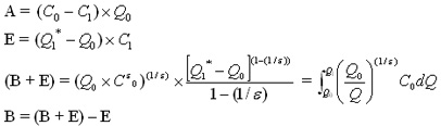
2.11 Additive Benefit Calculation MathematicsThe Highway Freight Logistics Reorganization Benefit Estimation Tool estimates the value of efficiency gains to the economy due to an industrial reorganization precipitated by a highway improvement. This appendix describes the mathematical process for estimating the efficiency gains that are estimated by the tool. The model calculates the change in demand for truck miles based on a change in price using the elasticity of demand with respect to price in the same manner.
The benefit estimation is driven by the estimation of total demand after the reorganization Benefit FactorThe benefit factor is the percent change in consumer surplus gained by the shift from D to
To assess the quantitative significance of the benefit factor, the tool contains or elicits quantitative evidence of the following:
For simplicity, this explanation focuses on how consumer surplus (A + B) is calculated for under demand D. Using the above equations and changing the Q and
The difference in benefit factor is determined by both The tool calculates the elasticity of demand with respect to the reorganization In order to calculate the change in demand from the reorganization, an estimate for the percent change in demand is calculated by multiplying
The benefit factor is then calculated by using
| ||||||||||||||||||||||||||||||||||||||||||||||||||||||||||||||||||||||||||||||||||||||||||||||||||||||||||||||||||||||||||||||||||||||||||||||||
|
United States Department of Transportation - Federal Highway Administration |
||