Comprehensive Truck Size and Weight Limits Study - Modal Shift Comparative Analysis Technical Report
Appendix D: Energy and the Environment Methodology
D.1 Scope
The purpose of this subtask is to evaluate the effect of alternative vehicle scenarios on the fuel consumption and greenhouse gas emissions of the fleet. The baseline vehicles and alternative configurations were evaluated on a range of drive cycles to determine their load-specific fuel consumption and emissions. The results of this analysis will be combined with modal shift data to represent the overall fuel consumption and emissions impact on the fleet.
D.2 Methodology
In previous truck size and weight studies such as the USDOT's Comprehensive Truck Size and Weight Study, 2000 (2000 CTSW Study), a simple table showing truck fuel economy in miles per gallon as a function of vehicle configuration and combined vehicle weight was used as an input to the energy and emissions analysis. For example, a triple 28-ft. trailer combination is listed as having 11 percent to 17 percent better fuel economy than that of a three-axle, 53-ft. box van trailer operating at the same vehicle weight. In practice, the 28-ft. triple-trailer combination suffers from higher aerodynamic drag than the 53-ft. box van trailer, and thus would be expected to have lower fuel efficiency.
The more recent OECD report "Moving Freight with Better Trucks" (OECD, 2011) uses fuel consumption values from road tests conducted by the German trucking magazine Lastauto Omnibus (page 152). These tests are run at maximum GCW over a defined route on German highways.
The approach selected for this study is to use baseline engine and vehicle models that are calibrated against experimental data and then modify the models to represent the range of vehicle scenarios selected for this project. This approach was first used in a 2009 report by the Northeast States Center for a Clean Air Future (Reducing Heavy-Duty Long Haul Combination Truck Fuel Consumption and CO2 Emissions, NESCCAF, 2009). The approach used here is also being used by the Southwest Research Institute (SwRI) in a study of fuel efficiency technologies being conducted for the National Highway Traffic Safety Administration (NHTSA). The models used in this project have been previously developed and verified as part of this NHTSA project.
The engine selected for this project is a 2011 model Detroit DD15. This is a widely used long-haul truck engine which has more than 20 percent of the long-haul market. The DD15 meets US EPA 2010 emissions requirements, and a slightly modified version of the engine has since been certified to meet the EPA's 2014 greenhouse gas requirements. From a proprietary benchmarking program, SwRI has an extensive set of performance, emissions, and fuel consumption data on this engine. Under the NHTSA contract, the experimental data was used to build and calibrate a GT-POWER simulation model of the engine. GT-POWER is a commercially available engine simulation tool. Four different ratings of the engine were developed in GT-POWER for this study: 428 HP, 485 HP (the baseline rating), 534 HP, and 588 HP.
The alternative engine power ratings were developed in order to maintain power-to-weight ratios for some of the alternative vehicle scenarios. For some scenarios, a much higher power would be required to maintain baseline vehicle performance. For example, if GCW is increased from 80,000 lbs. to 129,000 lbs., the baseline engine rating of 485 HP would need to increase to 782 HP in order to maintain the same vehicle acceleration and grade performance. Since engines over 600 HP are not available in the U.S. truck market, the decision was made to limit engine power to 588 HP and accept performance penalties for the highest vehicle weights.
The tractor selected for this study is a Kenworth T-700 high roof sleeper tractor. This truck is not offered with the DD15 engine, but it is offered with the Cummins ISX, another 15 liter engine with similar performance, emissions, and fuel consumption characteristics. Coast-down testing of the tractor with a 53-ft. box van trailer was performed by SwRI under an EPA project to obtain aerodynamic drag and rolling resistance characteristics of the tractor. The T-700 is an aerodynamic tractor using standard (not SmartWay) tires, and the baseline trailer has no aerodynamic or low rolling resistance features. This tractor-trailer combination represents approximately the average current fleet vehicle performance from an aerodynamic and rolling resistance perspective.
Vehicle simulation was performed using SwRI's Vehicle Simulation Tool. This software package is based on the National Renewable Energy Lab (NREL) Advisor vehicle simulation program, which has hundreds of users worldwide. SwRI's VST tool incorporates improvements to the original NREL component models, and provides enhanced functionalities in ways that allow the user to define each component of the vehicle. Each component's set of parameters is defined in a MATLAB scripting format that is used in conjunction with a Simulink model.
Another key factor in any analysis of vehicle fuel consumption and emissions is the drive cycle. For this study, four operational modes were evaluated:
1. Urban interstate / freeway operation
2. Rural interstate / freeway operation
3. Urban non-interstate / non-freeway operation
4. Rural non-interstate / non-freeway operation
Five drive cycles were combined to reflect each of the four operational modes. The drive cycles are summarized in Table D1.
| Cycle # | Cycle Name | Comments |
|---|---|---|
| 1 | WHVC | Same as in NHTSA project |
| 2 | Low Speed NESCCAF | Same time scale, speed multiplied by 60/68 |
| 3 | NESCCAF | Same as in NHTSA project |
| 4 | Urban / Suburban WHVC | First 1200 seconds of WHVC |
| 5 | GEM Urban (CARB) | Same as in NHTSA project |
Cycle 1 used the World Harmonized Vehicle Cycle (WHVC), which was developed by the United Nations as a chassis dynamometer emissions and fuel economy test procedure for trucks. The cycle includes three components: a low-speed cycle, a stop-and-go urban cycle, a medium-speed "rural" cycle with one stop, and a higher speed (55 mph maximum) freeway component. The "urban/suburban" WHVC in cycle 4 was created by truncating the cycle at the 1,200 second mark (out of 1,800 seconds total for the cycle).
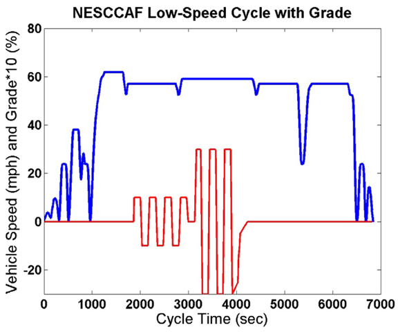
Cycle 2, the NESCCAF cycle (NESCCAF, 2009), had input from vehicle manufacturers, users, and regulators, and represents an attempt to simulate a U.S. long-haul duty cycle. There is some urban driving at the beginning and end of the cycle, with extended periods of high speed (65 to 68 mph) cruise, and some interruptions in speed designed to mimic a limited amount of traffic congestion. The cruise sections include periods of +/- 1 percent and +/- 3 percent grade.
The low speed NESCCAF cycle (cycle 2) is the exact same cycle but scaled down to limit the maximum speed to 60 mph.
Finally, cycle 5, the GEM Urban cycle, is the low-speed urban cycle used by the EPA in their Greenhouse gas Emissions Model, a simulation tool used to certify vehicles for compliance with the EPA's 2014 greenhouse gas emissions standards. This cycle was developed by the California Air Resources Board (CARB). Figures D-1 to D-4 show details of each drive cycle.
Figure D1. CARB urban cycle
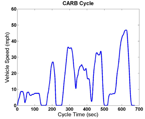
Figure D2. WHVC cycle
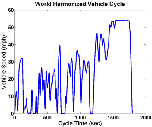
(The first 1200 seconds of the WHVC are used with the CARB cycle to simulate urban non-freeway driving. The full cycle is used to simulate urban freeway driving with congestion.)
Figure D3. NESCCAF Cycle with Grades
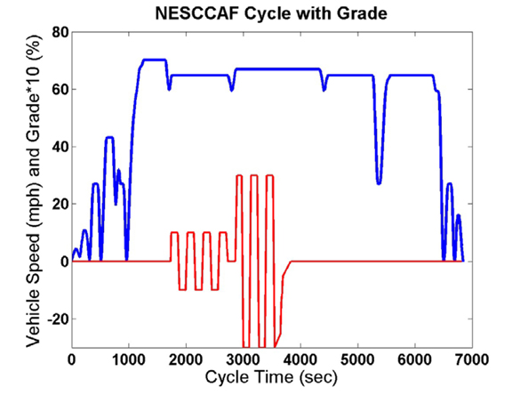
Figure D4. Low Speed NESCCAF Cycle with Grades
The drive cycles were combined to handle the four operational modes as shown in Table D2.
| Urban | Rural | Road Network |
|---|---|---|
| 50% WHVC, 50% Low Speed NESCCAF | NESCCAF | Interstate / Freeway |
| 50% Urban/Suburban WHVC, 50% Gem Urban | Low Speed NESCCAF | Non-Interstate / Non-Freeway |
A key difference between the 2014 and the 2000 CTSW Studies is that results are in terms of fuel consumption rather than fuel economy. In other words, the results are in terms of how many gallons of fuel it takes to move the vehicle a mile or to deliver a ton of freight 1,000 miles, or how many grams of emissions are emitted per vehicle mile or to move a ton of freight a mile. Differences in vehicle efficiency due to variations in tare weight and in aerodynamic drag are accounted for in this project's methodology. The results provided in this section will be combined with projected vehicle modal shift to provide predictions for the total fleet fuel consumption and emissions levels.
The fuel consumption methodology used in this project matches the methodology being used for the NHTSA study on fuel efficiency technologies being conducted by SwRI. This methodology has been reviewed with NHTSA, EPA, and in April 2014 with the National Research Council committee on Reducing the Fuel Consumption and Greenhouse Gas Emissions of Medium- and Heavy-Duty Vehicles, Phase 2.
For carbon dioxide (CO2) emissions, the study assumes that standard petroleum-based diesel fuel is used. There is a fixed relationship between a gallon of fuel and the amount of CO2 generated by burning it. 10.15 kilograms of CO2 are generated for every gallon of diesel fuel consumed.
For the purpose of this study, the study team assumes that all involved vehicles comply with 2010 EPA nitrous oxide (NOx) requirements of 0.2 grams per brake horsepower-hour, with a 10 percent engineering margin. Based on benchmarking tests performed by SwRI, this is a conservative assumption for the types of vehicle operation simulated for this project. The study team also assumes that brake-specific NOx emissions are independent of engine speed and load. Again, SwRI's internally developed benchmarking data shows this to be a reasonable assumption over a fairly wide range of speed and load. One additional assumption is required to allow a calculation of NOx emissions. For the 2014 CTSW Study, the study team assumed that the average brake specific fuel consumption of the engine over the drive cycles is 200 g/kW-hr. In actual practice, a range of 190 to 220 g/kW-hr can be expected. Using these assumptions, 3.8 grams of NOx can be expected for every gallon of fuel consumed.
Emissions Assumptions
For trucks complying with EPA 2010 and newer emissions standards, NOx emissions are roughly proportional to fuel consumption. Exceptions occur when vehicles are stuck in traffic congestion. Under these conditions, the exhaust system temperatures drop, and the selective catalytic reduction (SCR) NOx reduction system has degraded performance or, in extreme cases, ceases to function. Our analysis does not include operating scenarios where SCR performance is degraded, so we make the assumption that NOx is proportional to fuel consumption.
In order to calculate NOx, two assumptions are required. One is the estimated brake-specific fuel consumption (BSFC) of the engine in g/kW-hr over a drive cycle. Given the fuel map of the engine used in this study, we assumed a drive cycle average BSFC of 200 grams per kilowatt-hour. The next assumption is a NOx emissions rate of 0.24 g/kW-hr (0.18 g/HP-hr). This is a typical rate from 2010 and later certified engines, taken from public certification data available on the California Air Resources Board web site. Older engines will have a substantially higher NOx emissions rate, but for this study, we did not include the emissions characteristics of older engines.
Given the assumptions above, NOx emissions can be determined as follows:
0.24 g/kW-hr NOx / 200 g/kW-hr fuel consumption = 0.0012 g of NOx per gram of fuel
With 454 grams per pound, and a fuel density of 7 pounds per gallon of diesel fuel,
0.0012*454*7 = 3.8 grams NOx per gallon of fuel consumed
This rate was used with the fuel consumption results to determine grams of NOx per mile driven.
The calculation of CO2 per gallon of fuel depends only on fuel consumption and the hydrogen / carbon ratio of the fuel, since in a diesel engine, all available carbon can be expected to form CO2. From the US Energy Administration website, 1 gallon of diesel fuel yields 10.15 kg of CO2. As a result, the CO2 emissions (in kilograms) equals the fuel consumption in gallons/mile times a multiplier of 10.15.
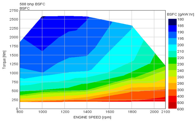
Engine Fuel Maps
A total of four engine ratings were evaluated: 428 HP, 485 HP (the baseline engine used for all vehicle scenarios), 534 HP, and 588 HP. For Scenarios 5 and 6, it is not practical to increase engine power enough to maintain performance. Scenario 6, with a weight limit of 129,000 lbs. would require 782 HP to have the same performance as the baseline 80,000-lb. vehicle with 485 HP. All four engine ratings were derived using the same 2011 model Detroit Diesel DD15 engine as the baseline, so engine displacement was not changed. This engine was thoroughly mapped by SwRI during a benchmarking project, and the experimental results were used to validate the GT-POWER engine model of the baseline 485 HP rating. The GT model was then used to develop the alternative ratings.
Figure D5. Fuel Consumption Map for the 428 HP Engine Rating.
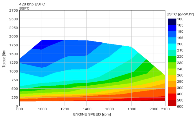
Figure D6. Fuel Consumption Map for the 485 HP (Baseline) Engine Rating.
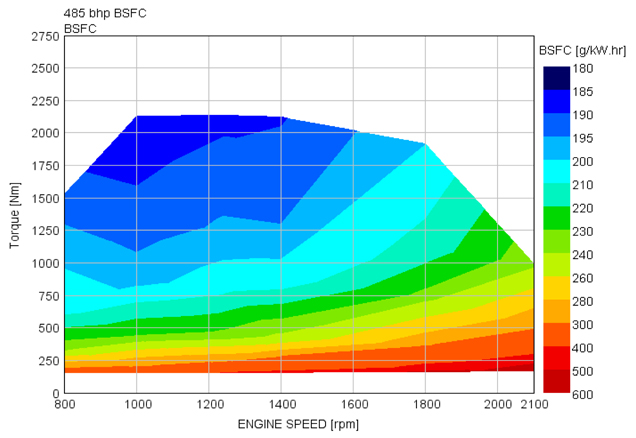
Figure D7. Fuel Consumption Map for the 534 HP Engine Rating.
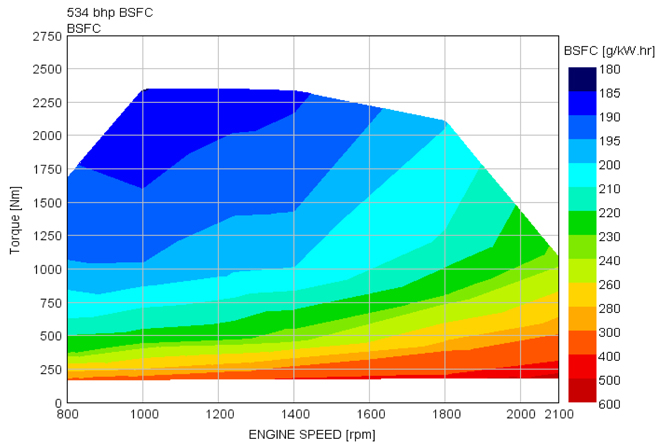
Figure D8. Fuel Consumption Map for the 588 HP Engine Rating.
Test Plan
For the vehicle baselines and for each vehicle scenario, fuel consumption and emissions were determined over a range of payload (and thus total vehicle weight). The range evaluated included zero payload (the truck at its empty weight), several payloads up to the maximum allowed weight for the vehicle scenario, and an overloaded vehicle weight of 200,000 lbs. The overloaded weight point was run to accommodate vehicles which run over the legal weight limit. The following vehicle configurations and payloads were evaluated:
A total of eight vehicle scenarios were run. Two of these vehicles represent the baselines: a five-axle 53-ft. trailer limited to 80,000 lbs., and a five-axle 28-ft. double-trailer combination, also limited to 80,000 lbs. The configurations evaluated are listed below in Table D3:
| Vehicle | Configuration | # Trailers | # Axles | Tare Wt. (Pounds) | Allowed GCW (lb) |
|---|---|---|---|---|---|
| A | 5-axle vehicle (3-S2) [baseline] | 1 | 5 | 34,622 | 80,000 |
| B | 5-axle vehicle (3-S2) | 1 | 5 | 34,622 | 88,000 |
| C | 6-axle vehicle (3-S3) | 1 | 6 | 36,255 | 91,000 |
| D | 6-axle vehicle (3-S3) | 1 | 6 | 36,255 | 97,000 |
| E | Tractor plus two 28-ft trailers (2-S1-2) [baseline] | 2 | 5 | 31,376 | 80,000 |
| F | Tractor plus two 33-foot trailers (2-S1-2) | 2 | 5 | 33,738 | 80,000 |
| G | Tractor plus three 28-foot trailers (2-S1-2-2) | 3 | 7 | 41,454 | 105,500 |
| H | Tractor plus three 28-foot trailers (3-S2-2-2) | 3 | 9 | 47,852 | 129,000 |
Each vehicle was simulated over a range of payloads, up to the maximum GCW. Vehicles that had maximum GCWs above 80,000 lbs. were evaluated with both the baseline engine and a higher rating intended to maintain performance or, in the case of Vehicles G and H, at least limit the performance penalty for the higher GCW. The payloads are shown in Table D4 below, along with the number of drive cycles evaluated and the total number of simulation runs required:
| Vehicle | Payloads To Be Simulated, Pounds | Engine Ratings | Drive Cycles | # Of Runs | ||||
|---|---|---|---|---|---|---|---|---|
| 1 | 2 | 3 | 4 | 5 | ||||
| A | 15,378 | 30,378 | 45,378 | 485 HP | All 5 | 15 | ||
| B | 15,378 | 30,378 | 45,378 | 53,378 | 485 HP, 534 HP | All 5 | 40 | |
| C | 15,378 | 30,378 | 45,378 | 54,745 | 485 HP, 534 HP | All 5 | 40 | |
| D | 15,378 | 30,378 | 45,378 | 60,745 | 485 HP, 588 HP | All 5 | 40 | |
| E | 15,378 | 30,378 | 45,378 | 48,624 | 485 HP, 428 HP | All 5 | 40 | |
| F | 15,378 | 30,378 | 46,262 | 485 HP | All 5 | 15 | ||
| G | 15,378 | 30,378 | 45,378 | 64,046 | 485 HP, 588 HP | 1, 2, 3 | 24 | |
| H | 15,378 | 30,378 | 45,378 | 64,046 | 81,148 | 485 HP, 588 HP | 1, 2, 3 | 30 |
In addition to the payloads shown above, each vehicle was also simulated under two additional conditions: a zero payload (empty vehicle) simulation and a GCW of 200,000 simulation. These two additional simulations for each vehicle along with the payload scenarios shown above allowed the CDM Smith team to estimate all possible emissions and energy consumption rates at all possible payloads for each vehicle analyzed. The final schedule of vehicle simulations according to GCW is shown on Table D5.
| Vehicle | Gross Combination Weight, Pounds | |||||||
|---|---|---|---|---|---|---|---|---|
| Allowed | 0 | 1 | 2 | 3 | 4 | 5 | 6 | |
| A | 80,000 | 34,622 | 50,000 | 65,000 | 80,000 | 200,000 | ||
| B | 88,000 | 34,622 | 50,000 | 65,000 | 80,000 | 88,000 | 200,000 | |
| C | 91,000 | 36,255 | 51,633 | 66,633 | 81,633 | 91,000 | 200,000 | |
| D | 97,000 | 36,255 | 51,633 | 66,633 | 81,633 | 97,000 | 200,000 | |
| E | 80,000 | 31,376 | 46,754 | 61,754 | 76,754 | 80,000 | 200,000 | |
| F | 80,000 | 33,738 | 49,116 | 64,116 | 80,000 | 200,000 | ||
| G | 105,500 | 41,454 | 56,832 | 71,832 | 86,832 | 105,500 | 200,000 | |
| H | 129,000 | 47,852 | 63,230 | 78,230 | 93,230 | 111,898 | 129,000 | 200,000 |
D.3 Findings
The result of these simulations were a set of rates describing the amount of fuel consumed and CO2 and NOx emitted from each vehicle at different payloads for each of the four operational modes. These rates were then applied to the weight specific VMT distributions developed by the modal shift analysis. Only those vehicles that were analyzed by the modal shift analysis were considered in the energy and emissions analysis. Other vehicles not a part of the modal shift analysis were not considered. The rates calculated are shown in Tables D6 through D29.
| Scenario | Urban Interstate / Freeway Gal/mile | ||||||
|---|---|---|---|---|---|---|---|
| 0 | 1 | 2 | 3 | 4 | 5 | 6 | |
| A | 0.124 | 0.141 | 0.158 | 0.176 | 0.339 | n/a | n/a |
| B | 0.124 | 0.141 | 0.158 | 0.176 | 0.185 | 0.339 | n/a |
| C | 0.126 | 0.143 | 0.160 | 0.178 | 0.189 | 0.341 | n/a |
| D | 0.126 | 0.143 | 0.160 | 0.178 | 0.196 | 0.341 | n/a |
| E | 0.128 | 0.144 | 0.161 | 0.178 | 0.182 | 0.338 | n/a |
| F | 0.130 | 0.146 | 0.163 | 0.182 | 0.341 | n/a | n/a |
| G | 0.143 | 0.159 | 0.177 | 0.193 | 0.215 | 0.351 | n/a |
| H | 0.149 | 0.167 | 0.184 | 0.202 | 0.223 | 0.242 | 0.358 |
| Scenario | Urban Interstate / Freeway Gal/mile | ||||||
|---|---|---|---|---|---|---|---|
| 0 | 1 | 2 | 3 | 4 | 5 | 6 | |
| A | 0.135 | 0.146 | 0.159 | 0.172 | 0.298 | n/a | n/a |
| B | 0.135 | 0.146 | 0.159 | 0.172 | 0.178 | 0.298 | n/a |
| C | 0.136 | 0.148 | 0.161 | 0.173 | 0.181 | 0.300 | n/a |
| D | 0.136 | 0.148 | 0.161 | 0.173 | 0.186 | 0.300 | n/a |
| E | 0.145 | 0.155 | 0.167 | 0.180 | 0.183 | 0.301 | n/a |
| F | 0.147 | 0.157 | 0.169 | 0.183 | 0.303 | n/a | n/a |
| G | 0.160 | 0.171 | 0.183 | 0.196 | 0.211 | 0.311 | n/a |
| H | 0.164 | 0.177 | 0.189 | 0.202 | 0.218 | 0.231 | 0.317 |
| Scenario | Urban Interstate / Freeway Gal/mile | ||||||
|---|---|---|---|---|---|---|---|
| 0 | 1 | 2 | 3 | 4 | 5 | 6 | |
| A | 1.26 | 1.43 | 1.61 | 1.78 | 3.44 | n/a | n/a |
| B | 1.26 | 1.43 | 1.61 | 1.78 | 1.88 | 3.44 | n/a |
| C | 1.28 | 1.45 | 1.63 | 1.80 | 1.91 | 3.46 | n/a |
| D | 1.28 | 1.45 | 1.63 | 1.80 | 1.99 | 3.46 | n/a |
| E | 1.30 | 1.46 | 1.63 | 1.81 | 1.84 | 3.44 | n/a |
| F | 1.32 | 1.48 | 1.66 | 1.84 | 3.46 | n/a | n/a |
| G | 1.45 | 1.62 | 1.79 | 1.96 | 2.18 | 3.56 | n/a |
| H | 1.52 | 1.70 | 1.87 | 2.05 | 2.26 | 2.46 | 3.64 |
| Scenario | Urban Interstate / Freeway Gal/mile | ||||||
|---|---|---|---|---|---|---|---|
| 0 | 1 | 2 | 3 | 4 | 5 | 6 | |
| A | 1.37 | 1.49 | 1.62 | 1.75 | 3.03 | n/a | n/a |
| B | 1.37 | 1.49 | 1.62 | 1.75 | 1.81 | 3.03 | n/a |
| C | 1.38 | 1.50 | 1.63 | 1.76 | 1.84 | 3.04 | n/a |
| D | 1.38 | 1.50 | 1.63 | 1.76 | 1.89 | 3.04 | n/a |
| E | 1.47 | 1.58 | 1.70 | 1.83 | 1.85 | 3.06 | n/a |
| F | 1.49 | 1.59 | 1.72 | 1.85 | 3.07 | n/a | n/a |
| G | 1.62 | 1.73 | 1.86 | 1.99 | 2.15 | 3.16 | n/a |
| H | 1.67 | 1.79 | 1.92 | 2.05 | 2.21 | 2.35 | 3.22 |
| Scenario | Urban Interstate / Freeway Gal/mile | ||||||
|---|---|---|---|---|---|---|---|
| 0 | 1 | 2 | 3 | 4 | 5 | 6 | |
| A | 0.47 | 0.54 | 0.60 | 0.67 | 1.29 | n/a | n/a |
| B | 0.47 | 0.54 | 0.60 | 0.67 | 0.70 | 1.29 | n/a |
| C | 0.48 | 0.54 | 0.61 | 0.68 | 0.72 | 1.29 | n/a |
| D | 0.48 | 0.54 | 0.61 | 0.68 | 0.74 | 1.29 | n/a |
| E | 0.49 | 0.55 | 0.61 | 0.68 | 0.69 | 1.29 | n/a |
| F | 0.50 | 0.56 | 0.62 | 0.69 | 1.29 | n/a | n/a |
| G | 0.54 | 0.61 | 0.67 | 0.74 | 0.82 | 1.33 | n/a |
| H | 0.57 | 0.64 | 0.70 | 0.77 | 0.85 | 0.92 | 1.36 |
| Scenario | Urban Interstate / Freeway Gal/mile | ||||||
|---|---|---|---|---|---|---|---|
| 0 | 1 | 2 | 3 | 4 | 5 | 6 | |
| A | 0.51 | 0.56 | 0.61 | 0.65 | 1.13 | n/a | n/a |
| B | 0.51 | 0.56 | 0.61 | 0.65 | 0.68 | 1.13 | n/a |
| C | 0.52 | 0.56 | 0.61 | 0.66 | 0.69 | 1.14 | n/a |
| D | 0.52 | 0.56 | 0.61 | 0.66 | 0.71 | 1.14 | n/a |
| E | 0.55 | 0.59 | 0.64 | 0.68 | 0.69 | 1.14 | n/a |
| F | 0.56 | 0.60 | 0.64 | 0.69 | 1.15 | n/a | n/a |
| G | 0.61 | 0.65 | 0.70 | 0.74 | 0.80 | 1.18 | n/a |
| H | 0.62 | 0.67 | 0.72 | 0.77 | 0.83 | 0.88 | 1.20 |
| Scenario | Urban Interstate / Freeway Gal/mile | ||||||
|---|---|---|---|---|---|---|---|
| 0 | 1 | 2 | 3 | 4 | 5 | 6 | |
| A | 0.190 | 0.196 | 0.226 | 0.256 | 0.588 | n/a | n/a |
| B | 0.190 | 0.196 | 0.226 | 0.256 | 0.273 | 0.588 | n/a |
| C | 0.194 | 0.199 | 0.229 | 0.260 | 0.279 | 0.590 | n/a |
| D | 0.194 | 0.199 | 0.229 | 0.260 | 0.291 | 0.590 | n/a |
| E | 0.186 | 0.191 | 0.220 | 0.250 | 0.257 | 0.580 | n/a |
| F | 0.191 | 0.196 | 0.225 | 0.257 | 0.583 | n/a | n/a |
| Scenario | Urban Interstate / Freeway Gal/mile | ||||||
|---|---|---|---|---|---|---|---|
| 0 | 1 | 2 | 3 | 4 | 5 | 6 | |
| A | 0.118 | 0.130 | 0.144 | 0.157 | 0.296 | n/a | n/a |
| B | 0.118 | 0.130 | 0.144 | 0.157 | 0.164 | 0.296 | n/a |
| C | 0.119 | 0.132 | 0.146 | 0.159 | 0.167 | 0.297 | n/a |
| D | 0.119 | 0.132 | 0.146 | 0.159 | 0.172 | 0.297 | n/a |
| E | 0.125 | 0.136 | 0.149 | 0.162 | 0.165 | 0.297 | n/a |
| F | 0.127 | 0.138 | 0.152 | 0.165 | 0.299 | n/a | n/a |
| Scenario | Urban Interstate / Freeway Gal/mile | ||||||
|---|---|---|---|---|---|---|---|
| 0 | 1 | 2 | 3 | 4 | 5 | 6 | |
| A | 1.93 | 1.99 | 2.29 | 2.60 | 5.96 | n/a | n/a |
| B | 1.93 | 1.99 | 2.29 | 2.60 | 2.77 | 5.96 | n/a |
| C | 1.97 | 2.02 | 2.32 | 2.64 | 2.83 | 5.99 | n/a |
| D | 1.97 | 2.02 | 2.32 | 2.64 | 2.96 | 5.99 | n/a |
| E | 1.89 | 1.94 | 2.23 | 2.54 | 2.61 | 5.89 | n/a |
| F | 1.93 | 1.98 | 2.28 | 2.61 | 5.92 | n/a | n/a |
| Scenario | Urban Interstate / Freeway Gal/mile | ||||||
|---|---|---|---|---|---|---|---|
| 0 | 1 | 2 | 3 | 4 | 5 | 6 | |
| A | 1.20 | 1.32 | 1.46 | 1.60 | 3.00 | n/a | n/a |
| B | 1.20 | 1.32 | 1.46 | 1.60 | 1.66 | 3.00 | n/a |
| C | 1.21 | 1.34 | 1.48 | 1.61 | 1.69 | 3.02 | n/a |
| D | 1.21 | 1.34 | 1.48 | 1.61 | 1.75 | 3.02 | n/a |
| E | 1.27 | 1.38 | 1.52 | 1.65 | 1.68 | 3.02 | n/a |
| F | 1.29 | 1.40 | 1.54 | 1.68 | 3.04 | n/a | n/a |
| Scenario | Urban Interstate / Freeway Gal/mile | ||||||
|---|---|---|---|---|---|---|---|
| 0 | 1 | 2 | 3 | 4 | 5 | 6 | |
| A | 0.72 | 0.74 | 0.86 | 0.97 | 2.23 | n/a | n/a |
| B | 0.72 | 0.74 | 0.86 | 0.97 | 1.04 | 2.23 | n/a |
| C | 0.74 | 0.76 | 0.87 | 0.99 | 1.06 | 2.24 | n/a |
| D | 0.74 | 0.76 | 0.87 | 0.99 | 1.11 | 2.24 | n/a |
| E | 0.71 | 0.73 | 0.84 | 0.95 | 0.98 | 2.20 | n/a |
| F | 0.72 | 0.74 | 0.85 | 0.98 | 2.22 | n/a | n/a |
| Scenario | Urban Interstate / Freeway Gal/mile | ||||||
|---|---|---|---|---|---|---|---|
| 0 | 1 | 2 | 3 | 4 | 5 | 6 | |
| A | 0.45 | 0.50 | 0.55 | 0.60 | 1.12 | n/a | n/a |
| B | 0.45 | 0.50 | 0.55 | 0.60 | 0.62 | 1.12 | n/a |
| C | 0.45 | 0.50 | 0.55 | 0.60 | 0.63 | 1.13 | n/a |
| D | 0.45 | 0.50 | 0.55 | 0.60 | 0.65 | 1.13 | n/a |
| E | 0.47 | 0.52 | 0.57 | 0.62 | 0.63 | 1.13 | n/a |
| F | 0.48 | 0.52 | 0.58 | 0.63 | 1.14 | n/a | n/a |
| Scenario | Urban Interstate / Freeway Gal/mile | ||||||
|---|---|---|---|---|---|---|---|
| 0 | 1 | 2 | 3 | 4 | 5 | 6 | |
| B | 0.12 | 0.141 | 0.159 | 0.176 | 0.186 | 0.345 | n/a |
| C | 0.13 | 0.143 | 0.161 | 0.178 | 0.189 | 0.346 | n/a |
| D | 0.13 | 0.144 | 0.161 | 0.179 | 0.197 | 0.353 | n/a |
| E | 0.13 | 0.144 | 0.161 | 0.178 | 0.181 | 0.331 | n/a |
| G | 0.14 | 0.160 | 0.178 | 0.195 | 0.217 | 0.365 | n/a |
| H | 0.15 | 0.168 | 0.186 | 0.204 | 0.225 | 0.246 | 0.373 |
| Scenario | Urban Interstate / Freeway Gal/mile | ||||||
|---|---|---|---|---|---|---|---|
| 0 | 1 | 2 | 3 | 4 | 5 | 6 | |
| B | 0.14 | 0.147 | 0.160 | 0.173 | 0.180 | 0.303 | n/a |
| C | 0.14 | 0.149 | 0.161 | 0.175 | 0.183 | 0.305 | n/a |
| D | 0.14 | 0.149 | 0.162 | 0.176 | 0.189 | 0.309 | n/a |
| E | 0.15 | 0.155 | 0.168 | 0.180 | 0.182 | 0.291 | n/a |
| G | 0.16 | 0.172 | 0.185 | 0.198 | 0.213 | 0.326 | n/a |
| H | 0.17 | 0.178 | 0.191 | 0.204 | 0.220 | 0.235 | 0.333 |
| Scenario | Urban Interstate / Freeway Gal/mile | ||||||
|---|---|---|---|---|---|---|---|
| 0 | 1 | 2 | 3 | 4 | 5 | 6 | |
| B | 1.26 | 1.43 | 1.61 | 1.79 | 1.89 | 3.50 | n/a |
| C | 1.28 | 1.45 | 1.63 | 1.81 | 1.92 | 3.51 | n/a |
| D | 1.29 | 1.46 | 1.63 | 1.82 | 2.00 | 3.59 | n/a |
| E | 1.30 | 1.46 | 1.63 | 1.80 | 1.84 | 3.36 | n/a |
| G | 1.46 | 1.63 | 1.80 | 1.98 | 2.20 | 3.70 | n/a |
| H | 1.53 | 1.70 | 1.89 | 2.07 | 2.29 | 2.49 | 3.79 |
| Scenario | Urban Interstate / Freeway Gal/mile | ||||||
|---|---|---|---|---|---|---|---|
| 0 | 1 | 2 | 3 | 4 | 5 | 6 | |
| B | 1.38 | 1.49 | 1.62 | 1.76 | 1.83 | 3.08 | n/a |
| C | 1.39 | 1.51 | 1.64 | 1.77 | 1.85 | 3.09 | n/a |
| D | 1.40 | 1.51 | 1.64 | 1.78 | 1.92 | 3.14 | n/a |
| E | 1.47 | 1.58 | 1.70 | 1.82 | 1.85 | 2.95 | n/a |
| G | 1.64 | 1.75 | 1.88 | 2.01 | 2.16 | 3.31 | n/a |
| H | 1.69 | 1.81 | 1.94 | 2.07 | 2.23 | 2.38 | 3.38 |
| Scenario | Urban Interstate / Freeway Gal/mile | ||||||
|---|---|---|---|---|---|---|---|
| 0 | 1 | 2 | 3 | 4 | 5 | 6 | |
| B | 0.47 | 0.54 | 0.60 | 0.67 | 0.71 | 1.31 | n/a |
| C | 0.48 | 0.54 | 0.61 | 0.68 | 0.72 | 1.32 | n/a |
| D | 0.48 | 0.55 | 0.61 | 0.68 | 0.75 | 1.34 | n/a |
| E | 0.49 | 0.55 | 0.61 | 0.67 | 0.69 | 1.26 | n/a |
| G | 0.55 | 0.61 | 0.67 | 0.74 | 0.82 | 1.39 | n/a |
| H | 0.57 | 0.64 | 0.71 | 0.77 | 0.86 | 0.93 | 1.42 |
| Scenario | Urban Interstate / Freeway Gal/mile | ||||||
|---|---|---|---|---|---|---|---|
| 0 | 1 | 2 | 3 | 4 | 5 | 6 | |
| B | 0.52 | 0.56 | 0.61 | 0.66 | 0.68 | 1.15 | n/a |
| C | 0.52 | 0.56 | 0.61 | 0.66 | 0.69 | 1.16 | n/a |
| D | 0.52 | 0.57 | 0.62 | 0.67 | 0.72 | 1.18 | n/a |
| E | 0.55 | 0.59 | 0.64 | 0.68 | 0.69 | 1.10 | n/a |
| G | 0.61 | 0.65 | 0.70 | 0.75 | 0.81 | 1.24 | n/a |
| H | 0.63 | 0.68 | 0.73 | 0.78 | 0.83 | 0.89 | 1.27 |
| Scenario | Urban Interstate / Freeway Gal/mile | ||||||
|---|---|---|---|---|---|---|---|
| 0 | 1 | 2 | 3 | 4 | 5 | 6 | |
| B | 0.191 | 0.197 | 0.226 | 0.257 | 0.274 | 0.604 | n/a |
| C | 0.195 | 0.200 | 0.230 | 0.260 | 0.280 | 0.606 | n/a |
| D | 0.196 | 0.201 | 0.231 | 0.261 | 0.293 | 0.624 | n/a |
| E | 0.185 | 0.190 | 0.220 | 0.250 | 0.257 | 0.561 | n/a |
| Scenario | Urban Interstate / Freeway Gal/mile | ||||||
|---|---|---|---|---|---|---|---|
| 0 | 1 | 2 | 3 | 4 | 5 | 6 | |
| B | 0.118 | 0.131 | 0.144 | 0.158 | 0.165 | 0.298 | n/a |
| C | 0.119 | 0.132 | 0.146 | 0.159 | 0.168 | 0.299 | n/a |
| D | 0.120 | 0.133 | 0.146 | 0.160 | 0.174 | 0.302 | n/a |
| E | 0.125 | 0.136 | 0.149 | 0.162 | 0.165 | 0.294 | n/a |
| Scenario | Urban Interstate / Freeway Gal/mile | ||||||
|---|---|---|---|---|---|---|---|
| 0 | 1 | 2 | 3 | 4 | 5 | 6 | |
| B | 1.94 | 1.99 | 2.30 | 2.61 | 2.78 | 6.13 | n/a |
| C | 1.98 | 2.03 | 2.33 | 2.64 | 2.84 | 6.15 | n/a |
| D | 1.99 | 2.04 | 2.34 | 2.65 | 2.98 | 6.34 | n/a |
| E | 1.88 | 1.93 | 2.23 | 2.54 | 2.61 | 5.69 | n/a |
| Scenario | Urban Interstate / Freeway Gal/mile | ||||||
|---|---|---|---|---|---|---|---|
| 0 | 1 | 2 | 3 | 4 | 5 | 6 | |
| B | 1.20 | 1.33 | 1.46 | 1.60 | 1.67 | 3.02 | n/a |
| C | 1.21 | 1.34 | 1.48 | 1.62 | 1.70 | 3.04 | n/a |
| D | 1.22 | 1.35 | 1.48 | 1.63 | 1.77 | 3.07 | n/a |
| E | 1.27 | 1.38 | 1.52 | 1.64 | 1.67 | 2.98 | n/a |
| Scenario | Urban Interstate / Freeway Gal/mile | ||||||
|---|---|---|---|---|---|---|---|
| 0 | 1 | 2 | 3 | 4 | 5 | 6 | |
| B | 0.73 | 0.75 | 0.86 | 0.98 | 1.04 | 2.29 | n/a |
| C | 0.74 | 0.76 | 0.87 | 0.99 | 1.06 | 2.30 | n/a |
| D | 0.74 | 0.76 | 0.88 | 0.99 | 1.12 | 2.37 | n/a |
| E | 0.70 | 0.72 | 0.84 | 0.95 | 0.98 | 2.13 | n/a |
| Scenario | Urban Interstate / Freeway Gal/mile | ||||||
|---|---|---|---|---|---|---|---|
| 0 | 1 | 2 | 3 | 4 | 5 | 6 | |
| B | 0.45 | 0.50 | 0.55 | 0.60 | 0.63 | 1.13 | n/a |
| C | 0.45 | 0.50 | 0.55 | 0.61 | 0.64 | 1.14 | n/a |
| D | 0.46 | 0.51 | 0.56 | 0.61 | 0.66 | 1.15 | n/a |
| E | 0.48 | 0.52 | 0.57 | 0.61 | 0.63 | 1.12 | n/a |
Rates were interpolated for each weight category for which modal shift VMT were provided. In total, there were 100 weight categories used in the modal shift analysis. Each weight category covered a 2,000-lb. range starting with 0 lbs. as the lower bound of the lowest category and ending with 200,000 lbs. as the upper bound of the highest category. The mid-point of each range was used as the average weight of the category. Rates were interpolated to the average weights of each category. The weight categories are shown in Table D30.
| Wt. Category | Min lb. | Max lb. | Mid lb. |
|---|---|---|---|
| 1 | 1 | 2,000 | 1,001 |
| 2 | 2,001 | 4,000 | 3,001 |
| 3 | 4,001 | 6,000 | 5,001 |
| 4 | 6,001 | 8,000 | 7,001 |
| 5 | 8,001 | 10,000 | 9,001 |
| 6 | 10,001 | 12,000 | 11,001 |
| 7 | 12,001 | 14,000 | 13,001 |
| 8 | 14,001 | 16,000 | 15,001 |
| 9 | 16,001 | 18,000 | 17,001 |
| 10 | 18,001 | 20,000 | 19,001 |
| 11 | 20,001 | 22,000 | 21,001 |
| 12 | 22,001 | 24,000 | 23,001 |
| 13 | 24,001 | 26,000 | 25,001 |
| 14 | 26,001 | 28,000 | 27,001 |
| 15 | 28,001 | 30,000 | 29,001 |
| 16 | 30,001 | 32,000 | 31,001 |
| 17 | 32,001 | 34,000 | 33,001 |
| 18 | 34,001 | 36,000 | 35,001 |
| 19 | 36,001 | 38,000 | 37,001 |
| 20 | 38,001 | 40,000 | 39,001 |
| 21 | 40,001 | 42,000 | 41,001 |
| 22 | 42,001 | 44,000 | 43,001 |
| 23 | 44,001 | 46,000 | 45,001 |
| 24 | 46,001 | 48,000 | 47,001 |
| 25 | 48,001 | 50,000 | 49,001 |
| 26 | 50,001 | 52,000 | 51,001 |
| 27 | 52,001 | 54,000 | 53,001 |
| 28 | 54,001 | 56,000 | 55,001 |
| 29 | 56,001 | 58,000 | 57,001 |
| 30 | 58,001 | 60,000 | 59,001 |
| 31 | 60,001 | 62,000 | 61,001 |
| 32 | 62,001 | 64,000 | 63,001 |
| 33 | 64,001 | 66,000 | 65,001 |
| 34 | 66,001 | 68,000 | 67,001 |
| 35 | 68,001 | 70,000 | 69,001 |
| 36 | 70,001 | 72,000 | 71,001 |
| 37 | 72,001 | 74,000 | 73,001 |
| 38 | 74,001 | 76,000 | 75,001 |
| 39 | 76,001 | 78,000 | 77,001 |
| 40 | 78,001 | 80,000 | 79,001 |
| 41 | 80,001 | 82,000 | 81,001 |
| 42 | 82,001 | 84,000 | 83,001 |
| 43 | 84,001 | 86,000 | 85,001 |
| 44 | 86,001 | 88,000 | 87,001 |
| 45 | 88,001 | 90,000 | 89,001 |
| 46 | 90,001 | 92,000 | 91,001 |
| 47 | 92,001 | 94,000 | 93,001 |
| 48 | 94,001 | 96,000 | 95,001 |
| 49 | 96,001 | 98,000 | 97,001 |
| 50 | 98,001 | 100,000 | 99,001 |
| 51 | 100,001 | 102,000 | 101,001 |
| 52 | 102,001 | 104,000 | 103,001 |
| 53 | 104,001 | 106,000 | 105,001 |
| 54 | 106,001 | 108,000 | 107,001 |
| 55 | 108,001 | 110,000 | 109,001 |
| 56 | 110,001 | 112,000 | 111,001 |
| 57 | 112,001 | 114,000 | 113,001 |
| 58 | 114,001 | 116,000 | 115,001 |
| 59 | 116,001 | 118,000 | 117,001 |
| 60 | 118,001 | 120,000 | 119,001 |
| 61 | 120,001 | 122,000 | 121,001 |
| 62 | 122,001 | 124,000 | 123,001 |
| 63 | 124,001 | 126,000 | 125,001 |
| 64 | 126,001 | 128,000 | 127,001 |
| 65 | 128,001 | 130,000 | 129,001 |
| 66 | 130,001 | 132,000 | 131,001 |
| 67 | 132,001 | 134,000 | 133,001 |
| 68 | 134,001 | 136,000 | 135,001 |
| 69 | 136,001 | 138,000 | 137,001 |
| 70 | 138,001 | 140,000 | 139,001 |
| 71 | 140,001 | 142,000 | 141,001 |
| 72 | 142,001 | 144,000 | 143,001 |
| 73 | 144,001 | 146,000 | 145,001 |
| 74 | 146,001 | 148,000 | 147,001 |
| 75 | 148,001 | 150,000 | 149,001 |
| 76 | 150,001 | 152,000 | 151,001 |
| 77 | 152,001 | 154,000 | 153,001 |
| 78 | 154,001 | 156,000 | 155,001 |
| 79 | 156,001 | 158,000 | 157,001 |
| 80 | 158,001 | 160,000 | 159,001 |
| 81 | 160,001 | 162,000 | 161,001 |
| 82 | 162,001 | 164,000 | 163,001 |
| 83 | 164,001 | 166,000 | 165,001 |
| 84 | 166,001 | 168,000 | 167,001 |
| 85 | 168,001 | 170,000 | 169,001 |
| 86 | 170,001 | 172,000 | 171,001 |
| 87 | 172,001 | 174,000 | 173,001 |
| 88 | 174,001 | 176,000 | 175,001 |
| 89 | 176,001 | 178,000 | 177,001 |
| 90 | 178,001 | 180,000 | 179,001 |
| 91 | 180,001 | 182,000 | 181,001 |
| 92 | 182,001 | 184,000 | 183,001 |
| 93 | 184,001 | 186,000 | 185,001 |
| 94 | 186,001 | 188,000 | 187,001 |
| 95 | 188,001 | 190,000 | 189,001 |
| 96 | 190,001 | 192,000 | 191,001 |
| 97 | 192,001 | 194,000 | 193,001 |
| 98 | 194,001 | 196,000 | 195,001 |
| 99 | 196,001 | 198,000 | 197,001 |
| 100 | 198,001 | 200,000 | 199,001 |
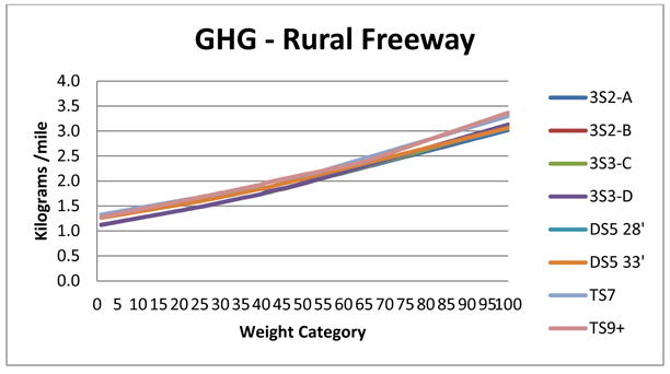
Rates for each weight category were interpolated through a simple method of linear interpolation considering the rates calculated during the vehicle simulations at each GCW. Example rate interpolations for rural fuel consumption and CO2 emissions are shown in Figures D9 to D10. Rates for all other road types and emissions were interpolated in a similar manner.
Figure D9. Rural Freeway Fuel Consumption
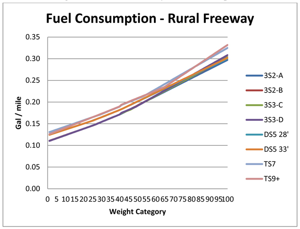
Figure D10. Rural Freeway CO2 Emissions
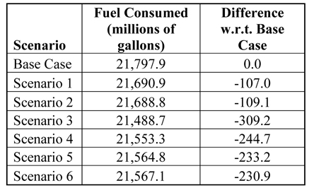
D.4 Fuel Consumption Results
Each scenario demonstrates reductions to fuel consumption relative to the Base Case scenario. This is consistent with the reduction of travel made possible by the increases in payload tested in each scenario. While most scenarios show comparable improvements, Scenario 3 shows the greatest overall reduction in fuel consumption. Tables D31-D38 show the changes to fuel consumption between each of the scenarios.
Table D31- Annual US fuel consumption (in gallons) for the Base Case in 2011.
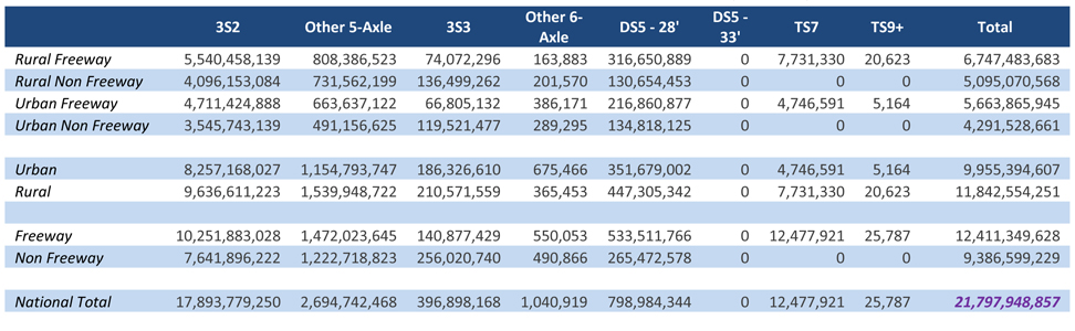
Table D32- Annual US fuel consumption (in gallons) for the Scenario 1 in 2011.
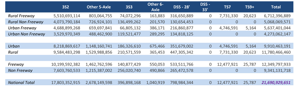
Table D33- Annual US fuel consumption (in gallons) for the Scenario 2 in 2011.
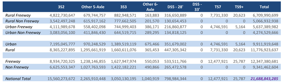
Table D34- Annual US fuel consumption (in gallons) for the Scenario 3 in 2011.
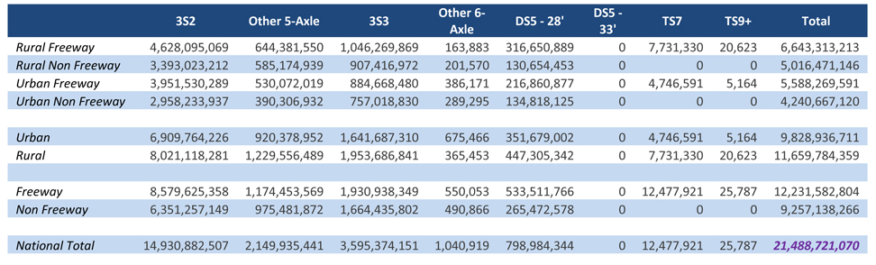
Table D35- Annual US fuel consumption (in gallons) for the Scenario 4 in 2011.
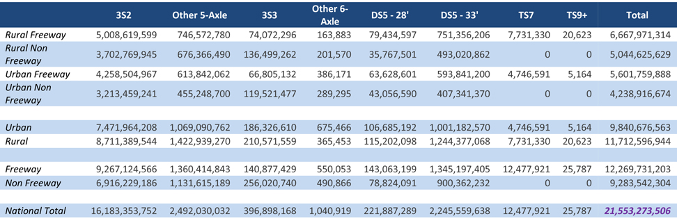
Table D36- Annual US fuel consumption (in gallons) for the Scenario 5 in 2011.
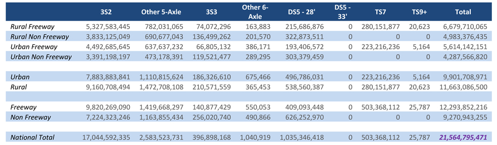
Table D37- Annual US fuel consumption (in gallons) for the Scenario 6 in 2011.
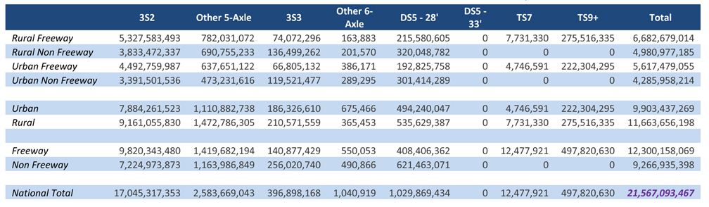
Table D38- Truck Fleet Annual Fuel Consumption.
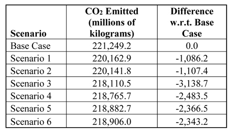
D.5 GHG Emissions Results
Each scenario demonstrates reductions to greenhouse gas emissions relative to the base case scenario. This is consistent with the reduction of travel made possible by the increases in payload tested in each scenario. While most scenarios show comparable improvements, Scenario 3 shows the greatest overall reduction in greenhouse gas emissions. Tables D39-D46 show the changes to CO2 emissions between each of the scenarios.
Table D39- Annual US Base Case CO2 Emissions (in kilograms).
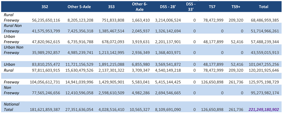
Table D40- Annual US Scenario 1 CO2 Emissions (in kilograms).

Table D41- Annual US Scenario 2 CO2 Emissions (in kilograms).
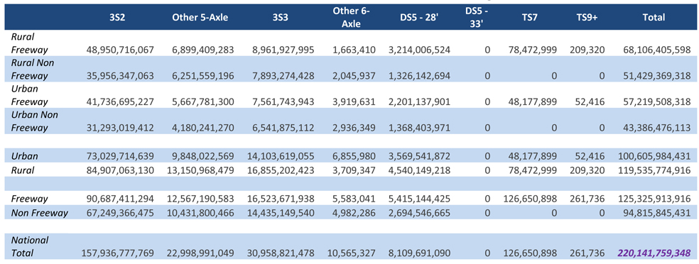
Table D42- Annual US Scenario 3 CO2 Emissions (in kilograms).
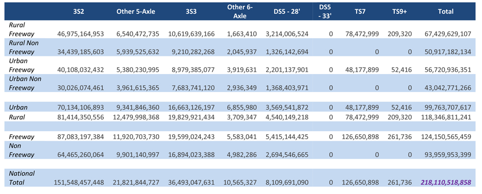
Table D43- Annual US Scenario 4 CO2 Emissions (in kilograms).
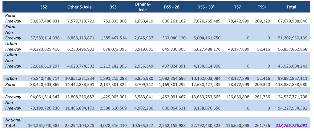
Table D44- Annual US Scenario 5 CO2 Emissions (in kilograms).
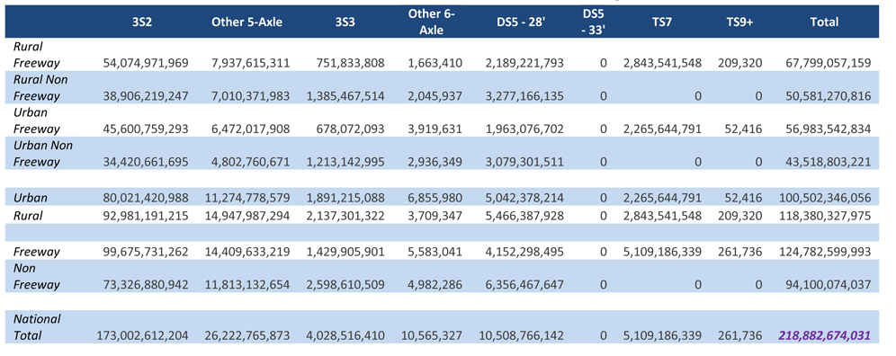
Table D45- Annual US Scenario 6 CO2 Emissions (in kilograms).
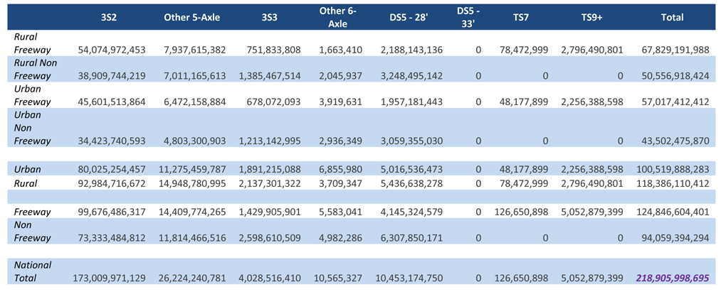
Table D46- Truck Fleet Annual CO2 Emissions.
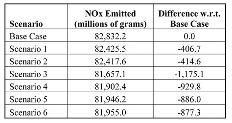
D.6 NOx Emissions Results
Each scenario demonstrates reductions to NOx emissions relative to the Base Case scenario. This is consistent with the reduction of travel made possible by the increases in payload tested in each scenario. While most scenarios show comparable improvements, Scenario 3 shows the greatest overall reduction in NOx emissions. Tables D47-D54 show the changes to NOx emissions between each of the scenarios.
Table D47- Annual US Base Case NOx Emissions (in grams).
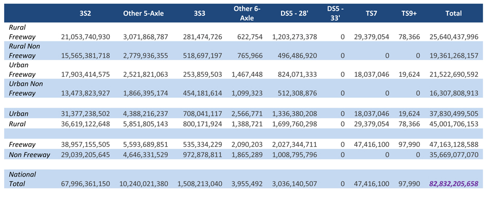
Table D48- Annual US Scenario 1 NOx Emissions (in grams).
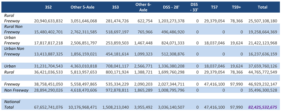
Table D49- Annual US Scenario 2 NOx Emissions (in grams).
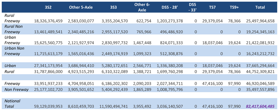
Table D50- Annual US Scenario 3 NOx Emissions (in grams).
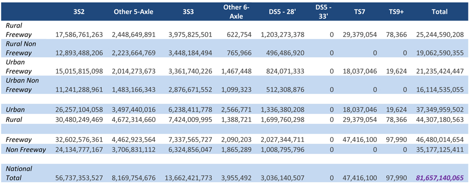
Table D51- Annual US Scenario 4 NOx Emissions (in grams).
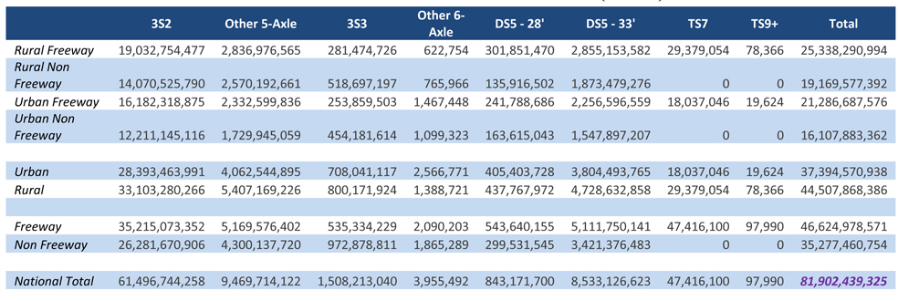
Table D52- Annual US Scenario 5 NOx Emissions (in grams).
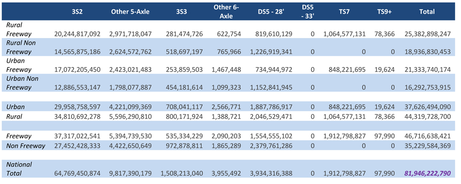
Table D53- Annual US Scenario 6 NOx Emissions (in grams).
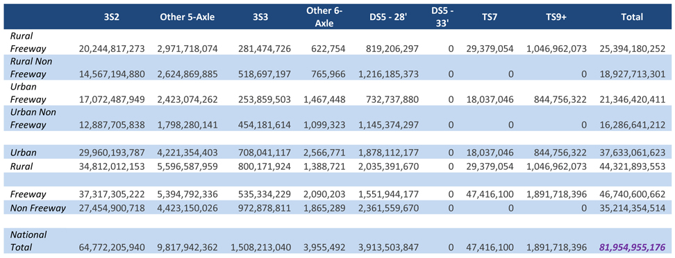
Table D54- Truck Fleet Annual NOx Emissions.
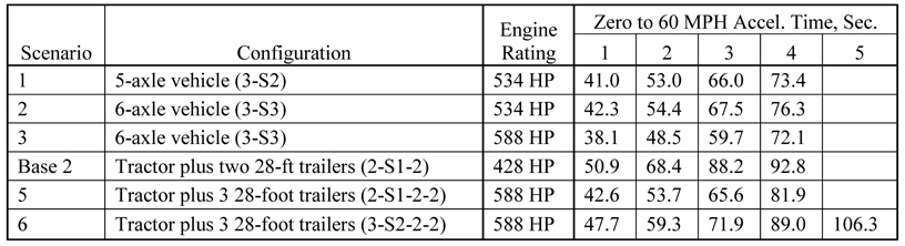
D.7 Vehicle Performance Results
Increases in allowed vehicle weight will naturally have an impact on vehicle performance. For this task, two metrics were evaluated. The first is the maximum speed that is achieved while the truck climbs a 3 percent grade. This speed is an indicator of how much a truck might slow traffic while climbing a grade. The second metric is 0 to 60 mph acceleration time, an indicator of how a truck might slow traffic when accelerating from a traffic light. Vehicle performance was evaluated both with the baseline 485 HP engine rating, and with alternative ratings.
In general, increasing maximum allowed vehicle weight will lead to a reduction in performance. This can be balanced by increased engine power, but at some weight, the truck will need more power than is currently available on the market. Since the highest rating currently available is 600 HP, our evaluation of alternative ratings stopped at 588 HP. The 588 HP rating can provide vehicle performance at 97,000 lbs., which matches the performance of the 80,000-lb. baseline vehicle with the baseline 485 HP engine. At 129,000 lbs., a 782 HP engine would be needed to match the baseline vehicle and engine performance. Note that performance values were not calculated for empty vehicles (payload 0) or overloaded vehicles (payload 6). In each table below, the highest payload evaluated represents the legal weight limit for that vehicle.
Table D55- Maximum Speed on 3% Grade with Baseline 485 HP Engine.
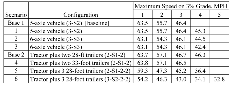
Table D56- Maximum Speed on 3% Grade with Alternative Engine Rating.
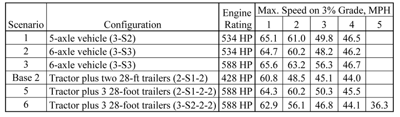
Table D57- Zero to 60 Mile Per Hour Acceleration Times with the Baseline 485 HP Engine.
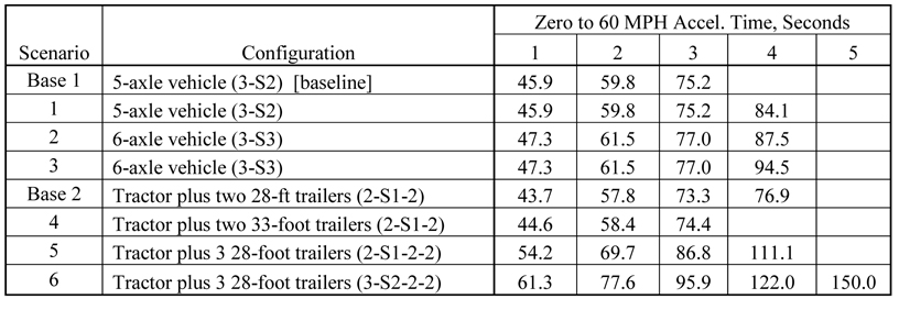
Table D58- Zero to 60 Mile Per Hour Acceleration Times with the Alternative Engine Ratings.
previous | next