Comprehensive Truck Size and Weight Limits Study - Modal Shift Comparative Analysis Technical Report
Chapter 3: Modal Shift Analysis and Results
This chapter summarizes data and methods included in the modal shift analysis and presents results of the analysis for each scenario. The discussion is organized around the various activities undertaken in conducting the modal shift analysis.
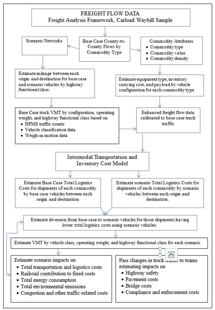
Figure 3 summarizes the overall modal shift analysis methodology. Basic elements of the methodology include the base case commodity flow data from the Freight Analysis Framework (FAF) and the Surface Transportation Board’s Carload Waybill Sample; the base case truck traffic volumes by vehicle class, highway functional class, and operating weight from the Highway Performance Monitoring System, state vehicle classification data, and state weigh-in-motion (WIM) data; commodity attributes from the latest (2002) Vehicle Inventory and Use Survey (VIUS) and other sources that affect the kind of equipment required to haul each commodity; the highway networks on which base case and scenario vehicles can travel; and the Intermodal Transportation and Inventory Cost (ITIC) model. Each of these elements is discussed in greater detail later in this Chapter.
From these data, transport and non-transport logistics costs for shipments of each of the 43 commodities included in the FAF between each origin and destination (approximately 3,000 counties in the United States) are calculated for applicable base case truck configurations, the scenario configuration, and for railroads. The model assumes that shippers choose the mode with the lowest total cost.
For a nationwide analysis such as this, it is impossible to include all factors that might affect mode choice decisions for individual moves, and the transport and non-transport cost factors included in ITIC can only be representative of actual costs for individual moves. However, these factors are believed to reflect the considerations that would affect long-term decisions on the choice of equipment for particular moves— especially for tradeoffs among the truck configurations—under the assumptions about each truck size and weight scenario.
Once the mode choice for each shipment has been estimated, overall changes in truck VMT and vehicle weight distributions can be estimated, as can changes in total transportation and logistics costs. Changes in overall energy consumption, environmental emissions, and traffic operations associated with changes in freight mode choice are also estimated in this study.
Impacts on pavements, safety, enforcement and compliance requirements, and bridge structures are estimated in the other studies within this volume:
- Pavement Comparative Analysis,
- Highway Safety and Truck Crash Comparative Analysis,
- Compliance Comparative Analysis, and
- Bridge Structure Comparative Analysis
Figure 3: Mode Shift Methodology
Analytical Assumptions and Limitations
In conducting the modal shift analysis, data and methodological limitations required the USDOT study team to make a number of assumptions:
- Cargo weighing less than 75,000 pounds GVW will not divert to six-axle (3-S3) tractor-semitrailers.
- Traffic currently moving in five-axle (3-S2) tractor-semitrailers that cannot benefit from the added weight allowed on a six-axle (3-S3) tractor-semitrailer will not shift to the six-axle vehicle. Simply put, carriers would not shift their entire fleets over to six-axle vehicles simply to increase the flexibility of their fleets.
- All scenario vehicles except triples have the same access to cargo origins and destinations as base case vehicles. This study assumes that, in the longer term, State and Federal agencies would make any necessary improvements to roads and bridges to enable these facilities to handle all scenario vehicles. The modal shift analysis is based on this long-term assumption.
- Triple configurations operate in LTL line haul (terminal to terminal) operations. In actuality there may be a few markets where heavy triples could be used for truckload shipments under the network and access restrictions placed on triples operations, but based on discussions with industry experts those are believed to be localized and would have very little impact nationally.
- Equipment currently being hauled in specialized configurations such as truck-trailer combinations will not shift to scenario vehicles. Specialized configurations are used because of unique commodity characteristics that would not be met by the scenario vehicles.
- Some 90 percent of short-line carloads interline with Class 1 railroads and thus are reflected in the Surface Transportation Board’s Carload Waybill Sample.
- The analysis year for the 2014 CTSW Study is 2011. To the maximum extent possible all data used for the study are from 2011 or have been adjusted to reflect 2011 values.
- The analysis assumes Federal and State highway user fees on the scenario vehicles are unchanged.
In addition to these assumptions, several other data limitations affect the analysis including:
- The precise origins and destinations of shipments are unknown from the FAF. Origins and destinations are assumed to be county centroids for inter-county shipments.
- The precise routes used to ship commodities between origin and destination are unknown. Shortest path routes between each origin and destination pair are calculated for purposes of estimating transportation costs.
- Physical characteristics of specific commodities within broad commodity groups may vary significantly.
- Shipment sizes and annual usage rates for freight flows between individual origins and destinations cannot be discerned from the FAF and must be estimated from VIUS and other sources. This affects non-transportation logistics costs.
- Rail carload and truck/rail intermodal origins and destinations are unavailable from the Carload Waybill Sample and have been estimated using the same assumptions as were used in the 2000 CTSW Study.
- Multi-stop truck moves to accumulate and distribute freight from and to multiple establishments are not captured in the FAF.
3.1 Freight Flow Data by Commodity, Origin-Destination, and Mode
Scope
Freight flow data are essential for estimating potential mode shifts associated with the truck size and weight variations studied under scenarios 1 through 6. Transportation characteristics and the requirements of different commodities vary significantly, but the coverage of all major commodities and all major transportation flows was an important criterion in choosing the commodity flow database to be used in this 2014 CTSW Study.
Another important consideration was the geographic detail of the origins and destinations. Some scenario vehicles cannot use all parts of the highway system, so the origin and destination granularity must be fine enough that differences in the networks available to scenario and base-case vehicles can be discerned. Finally public availability of both the data and any methods utilized to refine the data was an important element in scoping the study.
Methodology
As described in detail in the desk scan (Appendix A), the first step in this effort was to identify candidate commodity flow databases for use in this analysis. Four potential databases were identified: the FHWA’s FAF, the Commodity Flow Survey conducted by the Bureau of the Census, the Transearch database developed by IHS Global Insight, and the Surface Transportation Board’s Carload Waybill Sample for railroads.
Off the shelf, none of these databases met all the scoping considerations noted above, but the FAF came closest with respect to truck commodity flow data. The main weakness of the FAF data was that the geographic granularity was too coarse to allow differences in network availability for the different scenario vehicles to be evaluated. This issue was resolved for this study, with some loss of fidelity, when FHWA commissioned the Oak Ridge National Laboratory (ORNL) to disaggregate the FAF from its 123 regions to a county level of detail. Thus origins and destinations of commodity shipments between each of the approximately 3,000 counties in the country could be analyzed, creating a matrix of 9 million potential origin-destination pairs. The methodology used by ORNL to disaggregate the FAF data is included in Appendix A.
The commodity flow data for truck shipments in this 2014 CTSW Study is superior to the truck database used in USDOT’s 2000 CTSW Study. The FAF was not available when the 2000 CTSW Study was underway. At that time the only available database that met the study’s needs was the National Truck Stop Survey (NATS) conducted by the Association of American Railroads. The NATS had other weaknesses as compared to the FAF, including the fact that it had many fewer observations and it was limited to long-haul shipments where drivers stopped at truck stops while traveling to their destinations and were willing to participate in the survey.
Results
The outputs of this effort are matrices of freight flows by commodity, origin and destination, and mode. The USDOT study team used data from the Surface Transportation’s Carload Waybill Sample to analyze potential shifts from rail to truck rather than the rail data in the FAF because the Carload Waybill Sample data include more detailed origin, destination, and other shipment characteristics than rail data in the FAF. The Carload Waybill Sample data also include information as to the rates paid for each move.
Forty-three Standard Classification of Transported Goods (SCTG) groups are included in the FAF. The Census Bureau defines SCTG Codes at a 5-digit level of detail, but also groups commodities into two-digit groups as well. The two-digit level of detail is used in the FAF. Table 2 shows the ton-miles of each commodity group shipped in five-axle tractor-semitrailers in 2011 as estimated from the FAF. The five-axle tractor-semitrailer is the base vehicle for scenarios 1-3 and also accounts for a significant share of LTL traffic analyzed in scenarios 4-6.
Source: Freight Analysis Framework
Table 3 shows the distribution of highway shipments by length of haul. Almost one-third of shipments contained in the FAF are 50 miles or less in length. Fewer than 10 percent of shipments are greater than 500 miles. The length of haul affects costs associated with using different modes and different types of equipment.
| Length of Haul (miles) | Percent of Trips |
|---|---|
| 0-50 | 30 |
| 51-100 | 18 |
| 101-250 | 28 |
| 251-500 | 15 |
| 501-1,000 | 6 |
| >1,000 | 3 |
Source: Based on 2011 Freight Analysis Framework
3.2 Estimation of Shipment Size for Each Shipping Alternative
Scope
The FAF contains annual flows of commodities between various origin-destination (O-D) pairs. These annual flows must be translated into the number of individual truck or rail shipments that would be required to haul these annual flows using different types of equipment.
Methodology
The VIUS provides information on the payload for each vehicle configuration. Likewise, information is available on the maximum payload that can be carried in different types of rail equipment. Dividing the annual tons of each commodity going between each O-D pair for each equipment type provides the total number of trips that would be required to haul the freight for each type of equipment.
Results
The output of this task is incorporated into ITIC to provide the ability to estimate the total number of loads required to move the annual tonnage of each commodity hauled between each O-D pair by each type of truck and railroad equipment.
3.3 Freight Assignment to Highway Equipment, Including: Body Type, Configuration and Payload
Scope
Commodity characteristics are important determinants of the types of equipment that would be used and the payloads for shipments of each commodity. Among the most important commodity characteristics for the mode shift analysis are density, physical characteristics of the commodity, value, and the origin and destination of the shipment.
Commodity density measured in pounds per cubic foot directly influences whether a commodity will fill the cubic capacity of a trailer or container before the maximum payload is reached (a “cube-out” commodity) or whether the maximum payload will be reached before the trailer or container is physically filled (a “weigh-out” commodity). This, in turn, determines the extent to which a commodity could take advantage of potential changes in truck size and weight limits. Cube-out commodities generally would not benefit from increases in the allowable weight of a vehicle if the vehicle’s cubic capacity were not increased. Likewise, weigh-out commodities would not benefit by increases in the cubic capacity of a vehicle if the maximum gross vehicle weight were not also increased.
For many commodities, physical characteristics dictate the types of equipment that could be used to carry the commodities. Bulk commodities are almost always shipped in vehicles with specialized body types designed to accommodate their size. For example, construction equipment, building materials, lumber, large spools of wire and other similar commodities that cannot easily be loaded in a dry van typically are moved on flatbed or other specialized trailer.
This analysis estimated the vehicle configurations and body types that could be used to transport various commodities. It also estimated the tare weights of each vehicle configuration and body type of interest from which maximum payloads were estimated.
Methodology
The primary source of information on the vehicle configurations and body types used to haul various commodities is the VIUS. As noted above, the last VIUS was conducted in 2002, but the basic types of equipment used to haul various types of commodities have not changed significantly since that survey. The VIUS asked specific questions concerning the vehicle configurations and body types used to haul different commodities. It also asked the percentage of miles a vehicle was fully loaded and empty. Based on responses to these questions and estimates of commodity density, a payload distribution was developed for each commodity and vehicle configuration.
As noted above, the commodity groups contained in the FAF are not homogeneous. Within each group there may be a range of different commodities with different densities and different physical characteristics that affect the body type used to haul those commodities. For each commodity group within the FAF the distribution of vehicle configurations, body types, and payloads was estimated based on information from the VIUS.
During the process of disaggregating FAF to the county level a number of O-D pairs had annual tonnage volumes for specific commodities below 25 tons. It is unclear whether such small shipments of individual commodities actually occurred, but it is highly unlikely that they were hauled in truckload lots. Rather than discard these observations, the moves were treated as LTL shipments regardless of the commodity. The average volume handled in this manner was 4 tons.
Tonnage for each commodity group was assigned to configurations (single unit trucks, truck trailer combinations, and single, double, and triple trailer combinations), number of axles, and equipment type (dry, bulk, open, refrigerated body types) based on the ton-mile weighted distribution of the commodity group reported in the 2002 VIUS. Likewise, VIUS data were used to estimate length-of-haul distributions (less than 100 miles, 100 to 200 miles, over 200 miles) for each commodity group.
Results
Figure 4 shows the estimated distribution of shipments in 2011 by body type for the two most prevalent tractor-semitrailer configurations, the 3-S2 (five-axle tractor semitrailer) and 3-S3 (six-axle tractor semitrailer). More than ten times as many shipments were made in the five-axle tractor-semitrailer than in the six-axle vehicle. The primary reason is that the five axle vehicle can carry the maximum Federal GVW limit on Interstate highways within current axle load limits and within the Federal Bridge Formula. There is no need for the additional axle that adds weight to the vehicle and increases fuel consumption as well. Within the 3-S2 configuration, bulk body types account for about half of all shipments, followed by dry vans (28 percent), flatbeds (14 percent), and refrigerated trailers (7 percent). This is not the same as the portion of registered trucks by body type. Because Figure 4 shows the rankings by number of shipments, it is skewed towards those body types that carry heavier commodities. Among the 3-S3 configurations, bulk trailers account for an even larger share of all loads (64 percent) followed by dry vans (22 percent) flatbeds (11 percent) and refrigerated units (3 percent). The large share of bulk trailers among 3-S3 configurations is consistent with the use of these vehicles to haul cargo at weights greater than typically are allowed on 5-axle vehicles. Many of these loads are hauled under special permit.
Figure 4: Current Distribution of Shipments by Body Type for Five- and Six-axle Tractor Semitrailers
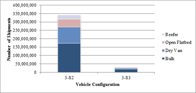
Table 4 shows the estimated tare (empty) weights of the vehicles analyzed in this 2014 CTSW Study. Many factors can affect a vehicle’s tare weight including where it operates (flat versus mountainous terrain), the construction of the trailer, whether the tractor has a sleeper and the dimensions of the sleeper, whether the vehicle has an auxiliary power unit to provide power when parked without having to run the engine, and whether the vehicle is equipped with dual or “super-single” tires. Thus the tare weights shown should be viewed as representative; weights of individual vehicles could vary.
NA = Not Applicable
(Scenarios 4, 5, 6 assume a non-sleeper cab-over-engine in dry van LTL operation – 3,000 pounds less weight than a conventional sleeper cab)
Tare, or unloaded, weights of different body types can vary significantly as shown in Table 4. On average, flatbed trailers are approximately 15 percent lighter than dry vans while refrigerated trailers and bulk trailers are estimated to be 6 percent and 7 percent heavier, respectively, than dry vans on average. Within these broad classifications, there may be additional variation; for example, bulk trailers include dumps, tanks, transit mixers, etc., each of which has a unique design and tare weight.
Table 5 shows the assumed payloads that can be carried by each of the scenario and base-case vehicles based on the tare weights. The maximum payload is simply the maximum gross vehicle weight minus the vehicle’s tare weight.
NA = Not Applicable
3.4 Calculation of Total Highway Travel by Configuration, Highway Network and Vehicle Operating Weight
Scope
An important input to the modal shift analysis is the base case distribution of travel by vehicle configuration, highway network, and operating weight. These data are needed not just for the modal shift analysis, but for all other tasks in this project. For the modal shift analysis the focus is on those vehicle configurations and weight groups from which freight traffic might divert to the scenario vehicles. Many truck configurations other than those selected for use in this study’s scenarios are in use today, but as previously noted, these generally have specialized uses, and traffic would not be likely to divert from those configurations to the scenario vehicles. Among the configurations not subject to significant diversion are tractor-semitrailers that already operate with more than six axles, truck-trailer combinations that have specialized uses, and twin trailers with more than five axles that would not be economical for LTL operations. This 2014 CTSW Study does not analyze the potential diversion of double-trailer dump construction vehicles. While some diversion might occur, it would have a small impact on national VMT because these are principally short-haul vehicles. Methods used to estimate base-case travel are described in detail in the Volume II: Data Acquisition and Technical Analysis Report.
Results
Table 6 shows VMT by vehicle configuration and operating weight. Data are shown only for the control vehicles for this study (five-axle semitrailers and twin 28’ trailers) and the scenario vehicle classes (six-axle tractor-semitrailer, seven-axle triple, and nine-axle triple). The Oth-CS5 designation represents a five-axle tractor-semitrailer with axles at the rear of trailer split by at least 8 feet. Note that for the purposes of this study, specifically for modelling impacts on pavement infrastructure, these split-axle sets were treated as a separate and different truck configuration. The Oth-CS5 variation appears in Tables 6-18 as a standalone configuration. No travel is shown for the twins with 33-foot trailers since that vehicle currently is not in wide use around the country.
The five-axle semitrailers have by far the greatest VMT of these vehicle classes. The split axles on the Oth-CS5 are considered single axles for weight enforcement purposes, allowing them to carry 20,000 pounds each under Federal axle load limits, compared to a total of 34,000 pounds that can be carried on the tandem axle of the 3-S2. Together the 3-S2 and the other CS5 traveled over 130 billion miles in 2011 compared with 2.4 billion for the six-axle tractor-semitrailer, 4.8 billion for twin 28-trailer combinations, and 222 million for triple trailer combinations. Among the triples, the seven-axle configuration dominates. That is the vehicle most frequently used in LTL operations. Triple-trailer configurations with nine or more axles account for less than 400,000 miles of total truck travel. Most of that travel is for the transportation of bulk commodities in the several States that allow those vehicles to operate at high weights.
Each configuration has considerable travel at weights above the Federal weight limit of 80,000 pounds on the Interstate System. Some of this occurs under special permit, some is allowed without special permit off the Interstate System in States where weight limits are higher than the Federal limits on the Interstate System. Some of the travel observed at weights above 80,000 pounds also represents illegal overloads. Shipping that uses by five- and six-axle semitrailers above 80,000 pounds would particularly benefit from the availability of the higher maximum vehicle sizes and weights being analyzed in this study, but LTL cargo that could use triples would also benefit.
Table 7 shows highway travel by vehicle configuration and functional highway system. The majority of travel by five-axle tractor-semitrailers (3-S2) and twin trailer combinations is on the Interstate System, but this is not true for other vehicle classes. More travel by six-axle tractor-semitrailers (3-S3) is off the Interstate System because they generally haul bulk commodities, and State weight limits often are higher off the Interstate System.
Data for the seven-axle and nine-axle triple trailers show considerable travel on lower order systems in both rural and urban areas, but those distributions are significantly affected by the limited operations of triple-trailer combinations. Several Western States allow triples to run widely off the Interstate System, but only a few Eastern States allow triples, and then only on turnpikes. Triples must assemble and disassemble immediately adjacent to the turnpike in those Eastern States.
Figure 5 shows the base case operating weight distribution for five- and six-axle semitrailers in 2011. The two five-axle combinations have peaks between 75,000 and 80,000 pounds, but the six-axle tractor-semitrailer has a much less pronounced peak at those weights. That vehicle travels substantial distances at weights above the 80,000 pound Federal limit.
Figure 6 shows the base case operating weight distributions for multi-trailer combinations. The twin trailer combination does not have a peak at the upper end of its weight distribution. Over half of its loaded travel is at weights at or below 60,000 pounds.
Figure 5: 2011 Base Case Operating Weight Distributions for Loaded Five and Six-axle Tractor-Semitrailers
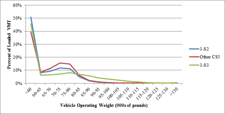
Figure 6: VMT 2011 Operating Weight Distribution for Loaded Twin 28-Foot Trailer and Triple Trailer Combinations
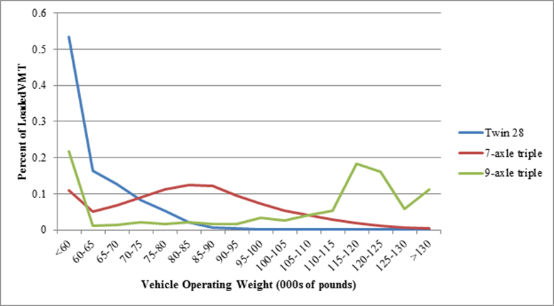
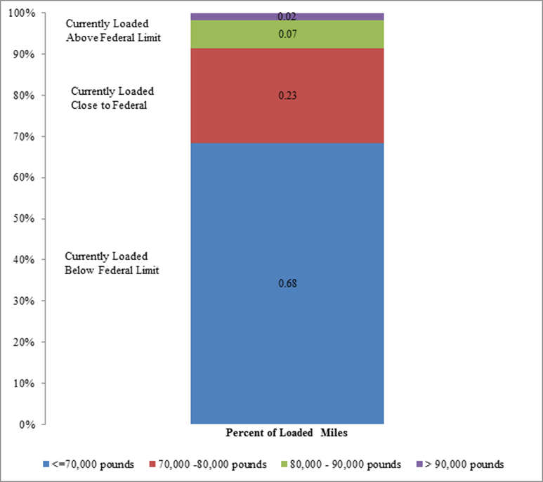
Figure 7 illustrates the share of VMT by five-axle (3-S2) tractor-semitrailers that potentially is susceptible to mode shifts if vehicles with higher GVW limits were allowed to operate. These vehicles travel more than 70 percent of total miles (and two-thirds of loaded miles) with operating weights of less than 70,000 pounds. These vehicles could load heavier but do not. Twenty-three percent of loaded 3-S2 VMT occur at operating weights between 70,000 and 80,000 pounds. These shipments could potentially benefit from higher weight allowances.
Figure 7: Share of Loaded VMT by 3-S2 that is Potentially Subject to Diversion
3.5 Calculation of Base Case Transportation Costs from Origin to Destination for Each Shipping Alternative
Scope
Truck rates are determined in large part based on the mileage between origin and destination, the equipment used to transport the shipment, and any special handling requirements to transport the commodity. In this subtask, transportation cost factors included in ITIC for base case and scenario vehicle configurations are updated and then applied to the FAF data on shipments of different commodities between different O-D pairs. These transportation costs, along with the non-transport logistics costs included in ITIC, are used to identify the most likely mode that would be chosen based on total logistics costs. Methods used are similar to those used in previous applications of ITIC by USDOT.
Methodology
The truck rate data used by FHWA in its last application of ITIC consisted of single trailer dry-van truckload rates for 113 market areas. Origins and destinations of the commodity flow database were mapped to one of the 113 markets in the truck rate database. One of the issues these rates reflect is existing lane imbalances, where head-haul/outbound rates higher than back-haul/inbound rates. The availability of more up-to-date rate information was examined, but no suitable truck rate databases were identified that were superior to the data last used by FHWA.
These market-based freight truckload rates were adjusted to account for several different factors including:
- Price differentials between dry-van trailers and specialized trailers (e.g. flatbed, tanker, refrigerated),
- Differences in empty-to-loaded ratios between dry-van and specialized trailers,
- The additional capital cost of multi-trailer configurations, and
- Overall changes in trucking costs between the year represented by the data and 2011, the base year for this analysis as reflected in the Producer Price Index for Transportation Services.
Differences in vehicle operating costs among the base case and scenario vehicles are important factors affecting the relative transportation costs of using different vehicle configurations. Among the vehicle operating cost components reflected in the ITIC model are cargo handling costs, line haul transportation costs, and pickup and delivery costs. These factors are specified for each vehicle configuration and body type analyzed in ITIC.
Similar cost components are included in the ITIC model for rail shipments. Among the rail cost elements are pickup and delivery costs, both per shipment and per mile. These costs vary for rail carload and TOFC/COFC moves. Revenues for shipments come directly from the Carload Waybill Sample.
The ITIC model was run against every record in the FAF database and the Carload Waybill database to estimate transportation costs by mode and vehicle configuration. This information was combined with estimates of non-transport logistics costs for each move to determine the mode and vehicle configuration with the lowest total logistics cost.
Results
The output of this effort is an updated ITIC model containing the most up-to-date data on the various transportation cost elements that affect mode choice decisions. Using these updated cost elements, costs were estimated for moves by base case and scenario vehicles of each commodity flow in the FAF and Carload Waybill Sample.
3.6 Calculation of Base Case and Scenario Non-Transport Logistics Costs for Each Shipping Alternative
Scope
Mode choice decisions are strongly influenced by non-transport logistics costs, including order cost, inventory carrying costs, storage, loss, and damage. In this subtask, non-transport logistic cost factors included in ITIC were reviewed, updated as necessary, and then applied to the FAF and Carload Waybill data on shipments of different commodities between different O-D pairs. These transportation costs, along with the non-transport logistics costs included in ITIC, are used to identify the most likely mode that would be chosen based on total logistics costs. The study ream used methods similar to those used by USDOT in previous applications of ITIC.
Methodology
Non-transport logistics costs in the ITIC model had been reviewed and updated by USDOT over the past few years so no major changes were required to the costs themselves.
For LTL operations, the USDOT study team opted to exclude non-transport logistics costs from the modal shift analysis since these vary primarily according to shipment size. Nothing in Scenarios 4-6—which analyzed vehicles primarily used for LTL shipments—would affect the size of individual shipments. The primary impact would be an increase in the number of shipments that could be hauled in a single trip.
For truckload freight, the study team calculated non-transport logistics costs for shipments of each commodity between each O-D pair and each potential mode. These non-transport logistics costs were combined with the transportation costs discussed in section 3.5 above to estimate total logistics costs for each move. These total logistics costs form the basis for estimating the choice of mode and vehicle configuration.
Results
The output of this sub-task is an estimate of non-transport logistics costs for moves of each commodity flow in the FAF and Carload Waybill Sample by base case and scenario vehicles.
3.7 Estimation of Total Logistics Costs and Scenario Impacts
Scope
This effort estimates the total logistics costs to move shipments of each commodity group between each origin and destination by base-case vehicles, railroads, and each scenario vehicle. The ITIC model selects the vehicle or mode with the lowest total logistics cost, including transportation costs and non-transport logistics costs. Each scenario involves only a single scenario vehicle. The ITIC model chooses either the base case vehicle/mode or the scenario vehicle. Results of the analysis of individual commodity movements between various origins and destinations are aggregated to estimate total changes from the base case that would occur if the scenario vehicle were allowed to operate.
Methodology
The analysis uses the ITIC model that has been described in preceding sections. Assumptions and limitations affecting the analysis are discussed above.
Results
Scenario 1
Scenario 1 would allow five-axle tractor semitrailers to operate at gross vehicle weights of 88,000 pounds. As discussed in the scenario descriptions, this vehicle could operate on the National Truck Network established in the Surface Transportation Assistance Act of 1982 and would have the same access off the network to reach terminals and facilities for food, fuel, rest, and repairs as the 80,000-pound, five-axle tractor-semitrailer currently operating widely in every State. For analytical purposes the USDOT study team assumes this vehicle to be able to travel directly to all origins and destinations identified in the FAF via the shortest path identified in the vehicle routing conducted for this study.
The primary impact of Scenario 1 would be to allow shipments currently moving in five-axle tractor-semitrailers to have a higher maximum GVW. For analytical purposes, the study team assumes that only truck traffic currently moving at weights above 75,000 pounds would be affected by this higher weight limit. Assuming that the same quantity of freight was transported under Scenario 1 as in the Base Case, allowing higher weights would reduce total travel since fewer trips would be required to haul the same quantity of goods.
Table 8 shows the overall change in VMT associated with increasing Federal weight limits for five-axle (3-S2) tractor-semitrailers from 80,000 pounds to 88,000 pounds and includes the Oth-CS5 designation, which represents a five-axle tractor-semitrailer with axles at the rear of trailer split by at least 8 feet. It is estimated that raising the Federal weight limit to 88,000 pounds for five-axle semitrailers would reduce total VMT by those vehicles by less than 1 percent. Few rail shipments shift to the heavier tractor-semitrailers analyzed in Scenarios 1-3. Those shipments that do shift from rail to truck under Scenarios 1-3 tend to be carload shipments that travel relatively short distances. Railroads, however, likely would have to reduce rates on many shipments to retain the freight traffic. This would have an adverse impact on their financial performance. Rail impacts are discussed in greater detail in Chapter 4.
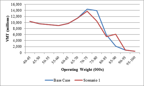
Figure 8 shows how the weight distribution for five-axle tractor-semitrailers is estimated to shift under Scenario 1. The peak at the current Federal weight limit of 80,000 pounds would disappear, but a new peak at about 88,000 pounds would appear. As noted, it is assumed that shipments currently operating at less than 75,000 pounds would not be affected by the higher weight limit.
Figure 8: Scenario 1 Shift in Weight Distribution for 5-axle Tractor Semitrailers
Scenario 2
Scenario 2 would allow a six-axle (3-S3) tractor-semitrailer to operate at a maximum GVW of 91,000 pounds on the National Truck Network with the same access to terminals and services off the network as a standard five-axle (3-S2) tractor-semitrailer with a maximum weight of 80,000 pounds. Shipments of bulk and other commodities that reach the vehicle’s maximum gross weight before filling the cubic capacity of the trailer would see the greatest benefit from this scenario. Shipping traffic for these items would potentially shift away from existing five-axle tractor-semitrailers, and the weight distribution of traffic currently operating in six-axle semitrailers would shift upward toward the 91,000 pound gross vehicle weight limit assumed in this scenario.
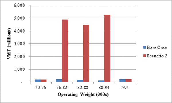
Table 9 shows the change in VMT for vehicle classes affected by the increased weight limits assumed under Scenario 2. Table 10 illustrates VMT change by operating weights.
Figures 9 and 10 illustrate graphically how freight traffic volumes at different operating weights change in Scenario 2 for 3-S2 and 3-S3 vehicle configurations. Beginning at the 76,000 to 82,000 pound weight range there would be large decreases in traffic for 3-S2 configurations and large increases in volume for 3-S3 configurations. Projections indicate that some shippers would continue to utilize the 3-S2 configuration at weights above 80,000 pounds due to permit operations and grandfathered State limits. Increases in 3-S3 traffic are particularly dramatic at weights above 80,000 pounds.
Figure 9: Scenario 2 Changes in 3-S2 Traffic by Operating Weight
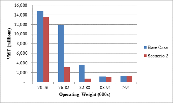
Figure 10: Scenario 2 Changes in 3-S3 Traffic by Operating Weight
Scenario 3
Scenario 3 is similar to Scenario 2 except the weight limit for six-axle tractor semitrailers is 97,000 pounds compared to 91,000 pounds in Scenario 2. The 97,000 pound 6-axle vehicle is assumed to be allowed on the entire National Truck Network and to have the same access off that network as current five-axle tractor-semitrailers.
Table 11 shows changes in total VMT for key vehicle configurations that could be expected under Scenario 3. Travel in the standard five-axle tractor-semitrailer is estimated to decrease by 14 percent while travel in the six-axle vehicle would increase by 700 percent. Total travel by these five- and six-axle semitrailers would decrease by 2 percent.
Table 12 shows changes in the operating weight distributions for key vehicle classes under Scenario 3. Figures 11 and 12 illustrate these changes graphically. As with Scenario 2, there is a significant shift of traffic from five- to six-axle vehicles. Projections indicate many freight shippers would be able to take advantage of the additional 6,000 pounds of payload under this scenario, contributing to a greater reduction in total VMT for Scenario 3 compared to Scenario 2.
Figure 11: Scenario 3 Change in 3-S2 Traffic by Operating Weight
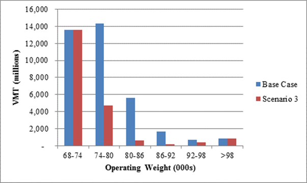
Figure 12: Scenario 3 Change in 3-S3 Traffic by Operating Weight
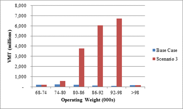
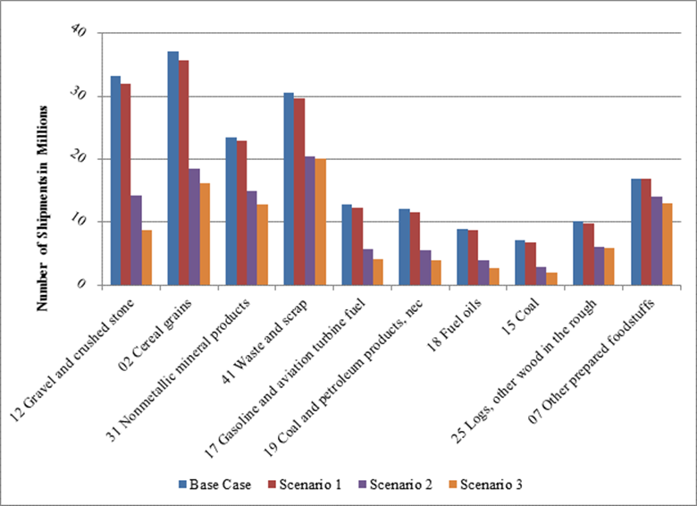
Figure 13 shows commodities that had the most shipments shift from the base case five-axle tractor-semitrailer to scenario vehicles and weights under Scenarios 1, 2, and 3. Most are bulk commodities that are hauled in various body types other than dry vans.
Figure 13: Changes in 3-S2 Shipments for Top 10 Commodities under Scenarios 1, 2, 3
Scenario 4
Scenario 4 analyzes the potential impacts of allowing twin 33-foot (2-S1-2) trailer combinations to operate at a maximum gross vehicle weight of 80,000 pounds. As noted in the scenario description, this analysis focuses on LTL cargo, including packages and mail. The twin 33-foot double trailers are assumed to operate on the same network as twin 28-foot doubles that are widely used for LTL operations today, and the new configuration would have the same access off that network to reach terminals and facilities for food, fuel, rest and repair.
Currently LTL over-the-road cargo is hauled primarily in five-axle tractor-semitrailers and twin 28-foot doubles. The FAF does not have a separate commodity group that includes all LTL shipments. The closest commodity group is mixed freight. In the analysis, mixed freight was used as a surrogate for LTL shipments with the recognition that shipments from other commodity groups also may be shipped in LTL operations. The VIUS differentiates LTL from TL shipments. Based on data from the VIUS, an estimated 17 percent of 3-S2 VMT is LTL traffic and 84 percent of 2-S1-2 traffic is LTL. The ITIC model was used to estimate the percentage of mixed cargo shipments that would shift from 3-S2 and 2-S1-2 (twin 28-foot doubles) configurations to the 2-S1-2 (twin 33-foot doubles) scenario vehicle. This percentage was applied to the portion of 3-S2 and 2-S1-2 (twin 28-foot doubles) traffic estimated to be used for LTL shipments.
Table 13 shows base case VMT for vehicles affected by truck size and weight changes analyzed in Scenario 4 and compares that VMT for those vehicle classes following shifts estimated under Scenario 4. The VMT for all other vehicle classes is assumed to be unaffected by changes under Scenario 4. Shifts to the twin 33-foot doubles from both five-axle semitrailers (including the 3-S2 and other CS5 configurations) and twin 28-foot doubles are estimated.
Table 14 summarizes the changes in truck traffic estimated to occur if twin 33-foot doubles were allowed. Reductions in five-axle tractor-semitrailer and twin 28-foot doubles traffic due to diversions to the twin 33-foot double configuration are estimated to total 16 billion miles while the new VMT for twin 33-foot doubles is estimated to total 13.1 billion miles. A net reduction of almost 3 billion miles would result from modal shifts under this scenario.
Approximately 15 million miles of the total 13.1 billion miles of twin 33-foot doubles traffic estimated under Scenario 4 is estimated to come from diversion of intermodal shipments from rail. The remainder would come from shifts in traffic from other truck configurations. The additional cubic capacity of the twin 33-foot doubles compared to existing twin 28-foot doubles is not enough to divert significant amounts of intermodal traffic from the railroads.
Scenario 5
Scenario 5 assumes that a seven-axle triple trailer (2-S1-2-2) would be allowed to operate on a 74,500 mile network of Interstate and other principal arterial highways at a maximum GVW of 80,000 pounds. Both Scenario 5 and Scenario 6 assume that, because of their length and other operating characteristics, triples’ access to roadways off the triples network would be limited to 2 miles. For analytical purposes, the USDOT study team assumed that if the origin or destination of a shipment is in a county through which the triples network passes, a terminal would be available within this 2-mile access distance. If the origin or destination of the shipment is not in a county through which the triples network passes, the triple configuration would have to be broken up, and twin trailers would have to be used until the triples network is available. Furthermore, for trips of less than 250 miles, the entire route would have to be on the triples network since it is assumed that the time necessary to break the triples into double trailers for drayage would render the diversion uneconomical. For trips longer than 250 miles it was assumed that a continuous distance of at least 250 miles on the triples network would be required before triples could be used. In practice, the relative costs of assembling and disassembling triples versus traveling the entire distance in doubles would vary from corridor to corridor depending on freight volume and shipper operations.
The assumption that triples would have very limited access to roadways off the triples network contrasts sharply with assumptions in USDOT’s 2000 CTSW Study, which assumed triples would have wide access off the network. The basic reason for changing the access assumptions for the current study was to portray a more realistic picture of how triples might actually be operated even if truck size and weight alternatives beyond those currently permitted were to be allowed. Whereas the 2000 CTSW Study attempted to estimate the maximum impact that various increased truck size and weight options might have, the assumptions in the current study are intended to more closely portray the realities of implementation. What this means is that if Federal law permitted, certainly some States might grant wider access than is being assumed in this study, but the USDOT study team judged it to be unlikely that many of the Eastern States would grant wide access off the network given the high traffic volumes and dense urban operating environments throughout large stretches of the northeast and southeast.
As shown in Table 6, seven-axle triples traveled an estimated 165 million miles in 2011. Almost all of these miles were accounted for by LTL operations, including package delivery. Triples operations are currently limited to a few Western States and on turnpikes in Kansas, Indiana, and Ohio. These configurations are attractive to LTL carriers because they offer 50 percent more cubic capacity than standard 28-foot doubles.
Table 15 compares base case VMT for the vehicle classes affected by Scenario 5 with an estimated VMT for Scenario 5 vehicles that would result from shifts associated with the assumed size and weight change under Scenario 5. There is a large shift of VMT to triples 2-S1-2-2, but there also is a net increase in the VMT for twin 28-foot doubles (2-S1-2). While some freight currently carried in twin 28-foot double trailers would shift to triples, the limited triples network means that some shipments shifting to triples must travel as doubles for part of the trip.
Table 16 summarizes changes by both VMT and weight group estimated to result from nationwide introduction of seven-axle triples (2-S1-2-2) at a maximum GVW of 105,500 pounds under network and access assumptions for Scenario 5. As noted in the discussion of Scenario 4, LTL operations currently use both five-axle tractor-semitrailers and twin trailer combinations. Triples offer significant increases in cubic capacity compared to both those configurations and also provide an increase in weight as well.
Under the Scenario 5 assumptions, triples traffic is estimated to increase from 165 million to over 3 billion miles annually based on 2011 freight volumes. Over 6.3 billion VMT would be diverted from five-axle tractor-semitrailers to triples operations, although not all of this travel would occur in triples. This 6.3 billion mile diversion of traffic represents almost 5 percent of total travel by five-axle tractor-semitrailers.
As noted above, triples cannot travel directly to all origins and destinations. Where the triples network does not directly serve origins and destinations, some of the freight traffic diverted to triples would have to travel in doubles. This accounts for the increase in doubles traffic shown in Table 16.
A significant portion of existing doubles traffic would also shift to triples under this scenario. Based on 2011 traffic volumes, an estimated 1.2 billion miles of 2-S1-2 travel would divert to triples. This represents approximately one-quarter of all 2-S1-2 traffic. The 1.2 billion miles of travel diverted from 2-S1-2 configurations would require only 810 million miles of travel by triples. The 1.2 million mile reduction in 2-S1-2 traffic and 810 million mile increase in triples traffic are included in Table 16.
The diversion of intermodal traffic from the railroads would result in about 11 million additional miles of travel by triples, which also is included in Tables 15 and 16.
The net reduction in total truck travel associated with Scenario 5 is estimated to be almost 2 billion miles, approximately 1.4 percent of total travel by 5-axle tractor-semitrailers, 5-axle doubles and 7-axle triples.
Scenario 6
Scenario 6 would allow nine-axle triple trailer combinations (3-S2-2-2) to operate on a 74,500 mile network of Interstate and other principal arterial highways at a gross vehicle weight of 129,000 pounds. While a small number of nine-axle triples currently operate in Western States, they primarily haul bulk commodities off the Interstate System. In nationwide operations, nine-axle triples could be expected to be used almost exclusively in LTL operations in much the same way that seven-axle triples (2-S1-2-2) operate today. The additional gross vehicle weight would allow them to carry heavier loads than they could under the 105,500 pound weight limit assumed in Scenario 5.
Table 17 compares total base case VMT for vehicles affected by Scenario 6 with VMT for those vehicles classes following shifts due to the size and weight changes assumed in Scenario 6. As with Scenario 5, traffic is shifted from five-axle tractor-semitrailers (3-S2) and twin 28-foot double configurations (2-S1-2) to the triple configuration (3-S2-2-2). Total twin 28-foot doubles traffic, however, increases as it did under Scenario 5 because triples cannot run from origin to destination for many of the shipments they haul. On portions of the route off the triples network, triples must break down and travel as doubles. Overall, VMT by vehicles affected by Scenario 6 is reduced by 1,944 million miles, 1.4 percent of the total base case travel by those vehicles classes.
About 6.3 billion VMT would be shifted from five-axle tractor semitrailers to triples and doubles under this scenario—about the same amount as shifted under Scenario 5. Despite this greater diversion, the nine-axle triples travel 6 percent fewer miles under Scenario 6 than the seven-axle triples do in Scenario 5. This reflects the additional GVW allowed on the nine-axle triples, which means fewer trips are required to carry those commodities that reach the 105,500 pound weight limit assumed in Scenario 5 before they fill the vehicle’s cubic capacity.
Table 18 shows the distribution of traffic shifts for Scenario 6 by operating weight. Most of the VMT shifting from the five-axle (3-S2) tractor-semitrailers is in relatively light weight groups. The greater cubic capacity of the triples allows them to carry more cargo at higher weights than is possible in tractor-semitrailers.
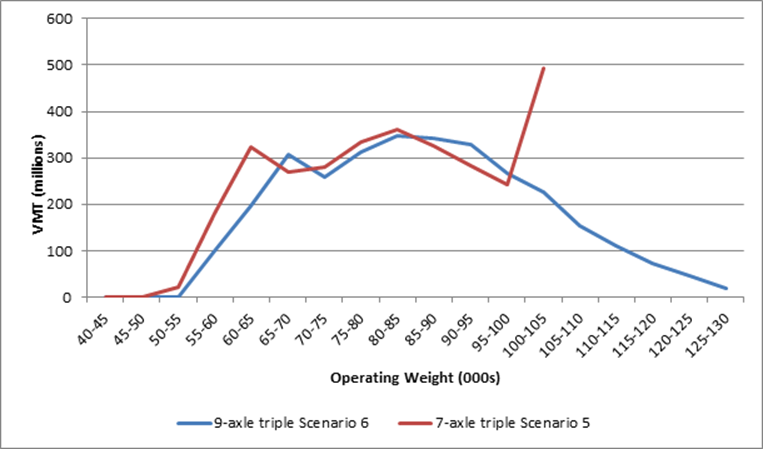
Figure 14 compares modal shifts to the triples configuration under Scenarios 5 and 6 by operating weight. In Scenario 5 there is a peak at the maximum GVW of 105,500 pounds, whereas in Scenario 6, which allows higher weight limits, the peak disappears and traffic is carried by the nine-axle triples at higher weights. The higher weight limits under Scenario 6 also result in fewer VMT being required to haul the traffic diverted from five-axle tractor semitrailers and 2-S1-2 configurations. The peak at the assumed maximum GVW for Scenario 5 results from the general assumption that traffic shifting to larger, heavier vehicles under the truck size and weight scenarios will not operate above the limits for each scenario. Traffic in scenario vehicles that currently operate above the scenario weight limit are assumed to continue to do so since they likely are operating under special permits that the study assumes would continue to be issued.
As was the case in Scenario 5, allowing triples actually increases total travel by 2-S1-2 configurations, despite the fact that considerable 2-S1-2 traffic shifts to the 9-axle triples. About 1.2 billion miles of 2-S1-2 travel shifts to triples under Scenario 6, resulting in an increase of 809 million VMT by triples. This is essentially the same amount of diversion from 2-S1-2 configurations that was estimated in Scenario 5. Offsetting the shifts of 2-S1-2 VMT to triples is the increase in 2-S1-2 VMT required to operate triples when the triples network does not directly connect origins and destinations. The increase in total diversion under Scenario 6 compared to Scenario 5 comes almost exclusively from 5-axle tractor-semitrailers that typically carry heavier loads than 2-S1-2 configurations.
Figure 14: Comparison of Traffic Shifts to 7 and 9-axle Triples by Operating Weight
As with Scenario 5, there is a small amount of diversion from intermodal rail to nine-axle triples under Scenario 6. Diversion from rail adds a total of 11 million miles of highway travel composed of 9.5 million in triples and 1.6 million in 2-S1-2 configured vehicles, which are required to complete moves where either the origin or destination is not on the triples network.
Table 19 shows the percentage of individual shipments that are estimated to shift from either 5-axle tractor-semitrailers or standard 28-foot doubles to the scenario vehicles for scenarios 4, 5, and 6 by shipment distance. At all trip distances virtually all LTL shipments in 3-S2 and 2-S1-2 vehicles are shown to shift to the twin 33-foot double configuration analyzed in Scenario 4. Little or no shift is expected to triple trailer combinations for shorter trip distances. The lack of diversion for trips less than 250 miles in length reflects the general assumption that shipments traveling less than 250 miles would not shift unless the entire trip could be made on the triples network. In specific corridors there could be exceptions to this assumption, but in general the additional handling costs of assembling and disassembling triples for such short trips would reduce the benefits of using triples. Virtually all LTL shipments traveling over 750 miles, however, would shift to triples from both single and double trailer combinations.
3.8 Cost Responsibility
The issue of cost responsibility often arises in connection with truck size and weight policy studies. Many truck size and weight options, including those examined in the current study, have highway investment implications, both in the near term and over time. These costs can be linked to changes in highway travel by different vehicle configurations at different weights as the result of the truck size and weight allowance changes. Many costs estimated in this study—including the pavement and bridge costs addressed later in this Volume II: Pavement Comparative Analysis and the Volume II: Bridge Structure Comparative Analysis—are related not just to operating weight but also to specific axle loadings for the various vehicle classes. To estimate the responsibility of different vehicle classes for changes in highway investment requirements, the distribution of axle loadings by vehicle classes affected by changes in truck size and weight allowances would have to be known.
Some have expressed interest in knowing how the impacts of truck size and weight allowance options might change if fees were imposed on trucks based on changes in their highway cost responsibility. Added fees would increase the relative cost of operating vehicles affected by different truck size and weight allowances and thus could affect the extent to which traffic shifts to those configurations from currently allowed configurations and from other modes. Estimating the fees that might be required to cover the added cost responsibility associated with different truck size and weight allowances would require an iterative process.
First, the added cost responsibility for each vehicle class affected by a modified size and weight allowance would have to be estimated under existing Federal and State highway user fees. Once the added cost responsibility was estimated, it would have to be translated into a cost per vehicle mile of travel for the affected vehicles. This additional cost would then have to be reflected in a new vehicle operating cost for each affected vehicle and the modal diversion and related impact analyses rerun to determine what changes charging vehicles for their additional cost responsibility in the first instance would have. Presumably the added cost responsibility would decrease and the additional user fee added to the second set of analyses would have to be adjusted to be closer in line with the new cost responsibility estimate.
While this type of analysis has some academic and policy interest, it also has real-world implications that should be considered. Primary among those is the fact that no single unit of government would likely see it as their responsibility to impose the full fee, since funding for operations and maintenance on the highways that would be most affected by truck size and weight allowance increases is a shared responsibility among Federal, State, and, in some cases, local governments.
In addition, there are implications for existing user fees. The most recent Federal highway cost allocation study and most State cost allocation studies have concluded that the user fees paid by operators of many heavy truck configurations currently are not adequate to cover their share of Federal or State highway cost responsibilities or their share of highway program costs. Imposing additional fees only on those vehicle classes responsible for changes in investment requirements associated with increased truck size and weight allowances raises questions concerning why user fees on other trucks should not be brought closer in line with their highway cost responsibility.
It is possible to address the cost responsibility issue purely through policy, in much the same way that the issue was addressed in the 1997 Federal highway cost allocation study, which noted the possibility or even desirability of taking a comprehensive look at overall highway user fee equity if truck size and weight limits were to be increased in such a way that significant additional highway investment might be required to accommodate the larger, heavier vehicles.
Nonetheless, a good starting point for discussion is presented in the Government Accountability Office study A Comparison of the Costs of Road, Rail, and Waterways Freight Shipments That Are Not Passed on to Consumers.[4] The study found that:
[F]reight trucking costs that were not passed on to consumers were at least 6 times greater than rail costs and at least 9 times greater than waterways costs per million ton miles of freight transport. Most of these costs were external costs imposed on society. Marginal public infrastructure costs were significant only for trucking.
This is a demonstration that trucking currently falls short of meeting its cost responsibility, especially with respect to damage inflicted on the highway infrastructure.
[4] United States Government Accountability Office, Report to the Subcommittee on Select Revenues Measures, Committee on Ways and Means, House of Representative, GAO-11-134, January 2011. Return to Footnote 4