ESTIMATING WORK ZONE DELAY AND QUEUE LENGTH PERFORMANCE MEASURES
Although queues and delays both characterize the same congested conditions at a particular work zone, they do represent different measures of congestion. Each type of measure can either be obtained directly from the data, or estimated using extrapolation procedures or fundamental relationships of traffic flow. For example, elapsed point-to-point travel times can directly measure delays, whereas field personnel can directly observe and record when and where the queue starts and ends. Conversely, spot speed sensors from a work zone ITS or from a functioning TMC can be extrapolated over segments of roadway to estimate travel times through a work zone.
In some jurisdictions, both types of data may be used to measure work zone mobility performance. While the use of different measures is not necessarily a problem for project-level evaluation, it can create a challenge for agencies wanting to use a single type of measure (or both measures) for program-level assessments. If this is the case, agencies will need to estimate the other types of performance measures from the data they have collected. Fortunately, this is fairly easy to accomplish, and steps to do so are covered in this section of the primer.
Two types of computations are described:
- Estimating travel time delays from manually-recorded queue length data, and
- Estimating travel time delays and queues from a series of spot sensors.
In addition, discussion is provided regarding the possible use of traffic simulation tools for estimating performance measures that are not monitored directly.
ESTIMATING DELAY FROM QUEUE LENGTH DATA
When queues form at a work zone, traffic speeds are significantly lower through the queue than upstream or downstream of the queue. The difference between the normal speeds on the facility and the reduced speed through the queue creates the delay that a motorist joining the queue experiences.
The process for estimating delay from manually-recorded queue length data is only appropriate for work zones in locations where recurrent congestion does not occur before a work zone is implemented so that assumptions can be made as to the speeds that would have existed prior to the installation of the work zone. Given these requirements, a simple three-step computation is all that is required to estimate delay from each queue length measurement recorded:
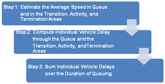
Figure 1. Steps to Estimate Travel Time Delays from Queue Length Data.
1. Estimate the Average Speed in Queue and in the Transition/Activity/Termination Areas
Queues result in travel time delays by creating slower speeds in both the queue and the transition/activity/termination areas of the work zone. If a queue has formed upstream of the lane closure bottleneck, it is first assumed that the flow rate through the work zone is at or near capacity. Given this assumption, speeds over the length of queue (Lq) are at the average speed in queue (Uq), and speeds over the length of the transition/activity/termination areas of the work zone (Lwz) are at the speed of capacity flow as illustrated below:
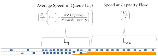
Figure 2. Components of Work Zone Delay.
Assuming a linear speed-density relationship, the speed at capacity flow through the transition/activity/termination areas can be computed simply as one-half of the free-flow speed (Uf) on the facility. Upstream of the work zone, the queue that develops will be flowing at a speed less than the capacity flow speed. Again using a linear speed-density relationship, the equation shown above produces an estimate of the average speed in queue as a function of the normal roadway capacity and the capacity through the work zone (WZ Capacity) (17) . The capacity of the work zone can be estimated using procedures in the Highway Capacity Manual (HCM) (18) . The HCM also provides procedures to estimate the normal capacity of the roadway segment. Typically, the following approximations will suffice:
- For 65- and 70-mph roadways: 2200 vehicles per hour per lane * number of lanes on the facility
- For 60-mph roadways: 2000 vehicles per hour per lane * number of lanes on the facility.
2. Compute Individual Vehicle Delay through the Queue and through the transition/activity/termination Areas
Assuming that the speeds computed in step 1 are maintained through the entire length of queue and work zone documented on the forms, estimates of average delays per vehicle through the queue and work zone can be computed. Travel at some threshold speed (most likely the desired speed or the posted work zone speed limit [UWZSL]) is used as the basis against which the longer travel times would be compared:
 (Equation 2)
If the activity area of the work zone is fairly long, congestion may not develop at the lane closure bottleneck as assumed above but at the location of the work zone activity due to driver rubbernecking or other factors. While speeds may slow significantly because of the increased distraction and lead to congested travel conditions within the work zone, speeds in that congestion will be operating closer to the speed at capacity flow than they will be to the estimated average speed in queue. Consequently, it is important to apply the correct speed estimate (speed at capacity flow, speed in queue) to the correct amount of the length of queue.
During a pilot test of work zone performance measures in Seattle, a lack of queue location documentation hampered efforts to accurately estimate motorist delays from queue length data. Estimated delays due to a 4-mile queue varied between 5.9 minutes if the queue were located entirely within the work zone lane closure, to 21.9 minutes if the queue were located entirely upstream of the work zone lane closure. At the Philadelphia pilot test site, the estimated delay for a 2.9-mile queue varied between 2.9 minutes and 29.8 minutes, depending on whether the queue was assumed to exist within or upstream of the work zone lane closure (2) .
Calculation of motorist delay from queue length data requires documentation of the amount of the queue located within the work zone and the amount that exists upstream of the work zone lane closure.
3. Sum Individual Vehicle Delays over the Duration of Queuing
Once the average delay per vehicle is estimated for each time interval that a queue is noted on the documentation form, the total vehicle-hours of delay is computed simply by multiplying the hourly volume by the average of the computed delay values at the beginning and ending of each hour. If the begin and end times of the lane closure and queue do not occur exactly on the hour, extrapolation techniques should be used to estimate the delays during that portion of an hour.
Typically, the manual documentation of queues at a work zone implies a lack of other traffic data collection devices available at the project, including hourly traffic volume data obtained while the work zone is in place. As a result, it may be necessary to rely on historical traffic volumes for these computations. If only AADT volumes are available, they will need to be distributed over the hours of the day to arrive at estimated hourly volumes.
The use of historical volumes for these (or any other volume-based) computations implies an assumption that 1) all traffic that normally used the facility before the work zone began continued to do so once the work zone was in place, or) any motorist who diverted experienced delays by using an alternative route that was equal to the delays being experienced by motorists remaining on the roadway and passing through the queue and the work zone.
ESTIMATING QUEUES AND DELAYS FROM SPOT SENSOR DATA
To estimate the queue length that exists at a work zone when spot speed traffic sensor data is used to monitor work zone mobility performance, it is necessary to evaluate traffic speeds over time and compare those speed patterns between adjacent sensors. In essence, the goal is to identify the discontinuity in traffic flow conditions between two adjacent sensors. The assumption made is that the beginning of the queue exists somewhere between those two sensor locations.
The process to estimate queue lengths and durations as well as travel time delays from spot sensor data consists of five basic steps:
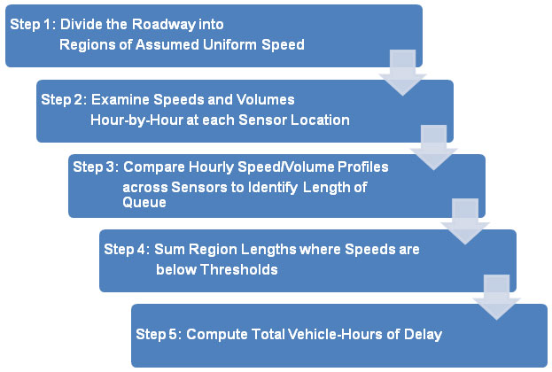
Figure 3. Steps to Estimate Queue Length and Delays from Spot Speed Sensor Data.
1. Divide the Roadway into Regions of Assumed Uniform Speed
In step 1, the roadway section where a work zone exists is divided into a series of segments of various lengths (L), with conditions in each segment assumed to be represented by its corresponding spot sensor data of volumes (V), average speeds (U), and detector occupancies (O) as illustrated below. Within each segment length, the travel time (TT) is estimated as the segment length divided by the average speed.
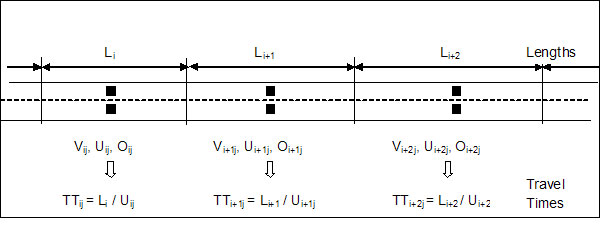
Illustration of Traffic Surveillance Estimates using Spot Sensor Data
2. Examine Speeds and Volumes Hour-by-Hour at each Sensor Location
To approximate queue lengths from spot sensors, the speeds at each sensor are examined in sequence and over time to identify the regions and times at each region in which speeds drop below a selected threshold. Speeds at successive sensor locations are examined together, and the length Li for each segment below the speed threshold is added together for each time interval of interest. In the example on the next page, spot traffic sensors are located 0.2 mile, 0.8 mile, and 1.3 miles upstream of the temporary lane closure. Project diary information indicates that a lane closure began at 9:00 AM and ended at 3:30 PM.
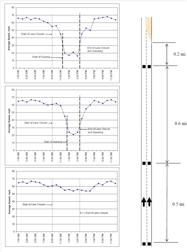
Figure 4. Example of Sensor Speed Analysis to Determine Duration and Length of Queue.
3. Compare Hourly Speeds across Sensors to Identify Extent of Queue Propagation
Starting with the downstream region, the average speeds over time at each region are examined in sequence moving upstream to estimate the upstream end of the queue each hour. For each hour (or other analysis period preferred by the agency), the objective is to identify how far upstream the queue has propagated. To accomplish this, the agency should select a speed threshold it will use to define the difference between normal traffic flow and traffic flow in a queue. This threshold can be defined as part of the agency’s work zone policy or procedures in absolute terms (e.g., speeds below 10 miles per hour, or speeds less than one-half of the free-flow speed of traffic on a facility), or in terms of the amount of reduction in speed observed by traffic approaching the work zone. Once a threshold is selected, it is a fairly simple task to determine the two regions in sequence that have a normal, high average speed at the upstream region and a low, congested speed indicative of the presence of queuing. The midpoint between the spot sensors of those two regions is where it is assumed that the upstream end of the queue is positioned during that hour. Performing this analysis hour-by-hour will result in a queue length profile over time at the work zone.
For the above example, a 40 mph speed threshold was selected as indicating queued traffic conditions. Consequently, the analysis of speeds at the upstream sensor locations indicates that a queue began to develop at approximately 11:30 AM at the first sensor, which grew upstream and reduced speeds at the second sensor at about 12:30 PM. The queue did not extend back to the third sensor, since speeds never did drop below 40 mph at that location during the hours of work activity. The estimated queue length each hour would therefore be as follows:
| Time | Estimated Location of Upstream End of Queue | Estimated Queue Length |
|---|---|---|
| 11:00 am | None | 0 |
| 12:00 pm | Between Sensors #1 and #2 | 0.2 + (0.6/2) = 0.5 mile |
| 1:00 pm | Between Sensors #2 and #3 | 0.2 + 0.6 + (0.5/2) = 1.05 mile |
| 2:00 pm | Between Sensors #2 and #3 | 1.05 mile |
| 3:00 pm | Between Sensors #2 and #3 | 1.05 mile |
| 4:00 pm | None | 0 |
4. Sum Travel Times across Sensors to Compute Individual Motorist Delay
The accuracy of both delay computations and queue length estimates using traffic sensor data are very dependent upon the distance between successive sensors. Estimation errors increase directly as the length between sensor increases.
As noted previously, the travel time at any point in time across a segment of roadway (TT) is simply the length of that region (L) divided by the speed at that point in time (U). Summing the individual travel times for each region together provides a total travel time over the length of roadway of interest at that point in time.
To estimate the work zone delay to an individual motorist approaching the work zone during a given hour, the travel times estimated in a pre-work zone condition are subtracted from those estimated from the speeds measured during the work zone over the same summed length of interest. As an alternative, a desired speed through the work zone can be defined and travel times based on that desired speed used to compare against actual work zone travel times. Such an approach might be used if the agency has posted a reduced speed limit through the work zone, and does not want delays measured against the normal, non-work zone speed limit and operating speeds.
5. Compute Total Vehicle-Hours of Delay
The final step in the process is to sum the individual motorist delays occurring each hour that queuing and congestion has developed. This is the average individual motorist delay each hour as computed in step 4, multiplied by the number of vehicles measured as traversing those regions during each hour, summed and converted to total vehicle-hours of delay.
USING A TRAFFIC SIMULATION MODEL TO ESTIMATE WORK ZONE PERFORMANCE MEASURES
Conceptually, it is also possible to use a traffic simulation model to estimate work zone performance measures not recorded directly through data collection efforts. Such an approach may be desirable, for example, if the agency had already developed a model for assessing potential impacts during work zone planning and design. An agency could gain valuable insights into the effectiveness of their design modeling efforts by revisiting the assumptions and data used and seeing how the resulting analysis compared to what occurred in the field.
A simulation model can also be used to estimate work zone performance measures that are not directly monitored in the field. To accomplish this, the model would first be calibrated to the pre-work zone conditions at a location. Then, the work zone would be added to the model, and the outputs calibrated to the conditions that were measured at the site. For example, if queue length and duration were measured through manual data collection methods, the model inputs and parameters would be adjusted systematically to match the documented queue patterns at the site. These adjustments may mean reducing or increasing the traffic volumes approaching the work zone or entering and exiting at various ramps upstream or within the work zone; adjusting the capacity values used for the normal roadway and for the work zone; or adjusting the geometric inputs to the model to modify the resulting capacity flows achieved through the simulated roadway section and the work zone. Once the queue patterns have been sufficiently replicated in the model, the output would provide the individual vehicle delays and total vehicle-hours of delay.
If this approach is used, it is important to correctly interpret and understand what the output from the model actually represents. For example, it may be necessary to significantly reduce the historical traffic volumes approaching the work zone in order to achieve the queue lengths observed in the field. This would imply that a significant amount of traffic diversion had occurred to other routes or travel modes. The estimates of individual motorist delay through the work zone could be fairly realistic, as they represent the delays incurred by a specific vehicle traversing a realistic length of queue and the work zone. However, if the simulation model did not include the alternative routes, the portion of traffic demand removed from the work zone would cause the vehicle-hours of delay to be underestimated by the amount of that removed traffic. Unless the agency is convinced that the diverted traffic experienced no additional travel time to their ultimate destinations, some means of accounting for diverted traffic delays would be necessary. Agencies would also need to assess how realistic the estimated diversion amounts are for the work zone of interest. If the calculated diverted traffic amounts are considered to be excessive for the roadway corridor, it would be necessary to further adjust some of the other parameters (work zone capacity, driver behavior parameters) to calibrate the model and extract the output results of interest.
previous | next