2.0 Data Collection and Preparation

Data collection is a critical step in the analysis process.  Knowing what to collect, when to collect, how long to collect, where to collect, and how to manage the data must be addressed before starting the collection.

This chapter provides guidance on the identification, collection, and preparation of the data sets needed to develop a CORSIM model for a specific project analysis, and the data needed to evaluate the calibration and fidelity of the model to real-world conditions present in the project analysis study area.  There are agency-specific techniques and guidance documents that focus on data collection, which should be used to support project-specific needs.  A selection of general guides on the collection of traffic data are listed on page 23 of Volume III.⁽⁷⁾  These sources should be consulted regarding appropriate data collection methods (they are not all-inclusive on the subject of data collection).  The discussion in this chapter focuses on data requirements, potential data sources, and the proper preparation of data for use in a CORSIM analysis.

If the amount of available data does not adequately support the project objectives and scope identified in Chapter 1, then the project team should return to Chapter 1 and redefine the objectives and scope so that they will be sufficiently supported by the available data.

Managing the data that is collected is critical to the success of the study.  It may be impossible to go back to collect data that was missed or lost if conditions have changed.  It is difficult to put confidence in data that was mishandled or its origins are not known.  Prior to beginning data collection, ensure that a data management system is in place and all personnel involved in the data collection know what the process is for collecting and storing the data.  If good management practices are in place, data will be less likely to be lost or corrupted.

Sources of data, times of traffic data collection, unusual events during collection, data collection decisions that were made, and time spent collecting and organizing should be documented.  By documenting the data collection while it is in progress, the final report becomes much easier to prepare.  The documentation can also be used to build historical data for future analysis project estimation.

Geometric, traffic demand (present and future), and signal data can be collected from many sources.  Collecting data for a traffic analysis may involve contacting many different agencies to obtain the data they maintain.  It is a good idea to assess what data are collected on an on-going basis or was collected recently for another analysis.  It may be possible to use existing data that is collected by planning organizations or from existing detectors from traffic management systems.  It is also a good idea to contact local agencies to make sure the traffic signal timings are not being updated or a large construction project is not scheduled to begin during the data collection period.  Some sources that may be contacted for data required for the analysis include:

• City or municipal street departments.
• County roadway departments.
• Regional council of governments.
• Planning agencies.
• State departments of transportation. 

In order to get current traffic data, it may be necessary to collect additional data that does not currently exist.  Additional data collection may involve tube-counters, radar speed measurement devices, turn count collection devices, and other methods mentioned in this chapter. 

Geometric data do not vary on a daily basis.  However, traffic and volume data does vary from day to day.  By collecting data on only one day, the data will likely not reflect the average traffic patterns.  Depending on the congestion and size of the study area, different sample periods should be collected.  The variability in the daily traffic will determine how long to collect data.  On lightly congested roadways it may be possible to collect only a few days worth of traffic data.  For projects with more significant congestion, a week or more of data collection may be needed.

All data should be collected during the same time frame if possible.  If all the data are not collected over the same time frame, there may be problems resolving data inconsistencies or in calibrating the model.  For example, collecting mainline volume data during one week and collecting turning data during the next week may result in turning data that are difficult to match with the mainline volume data. 
Data should be collected during peak or off peak periods when typical traffic conditions exist.  Traffic data collection should be avoided during such conditions as during incidents, inclement weather, special events, construction, holidays and seasonal variations (unless these special conditions are part of the analysis purpose).

A good storage process is critical to the success of the analysis.  For easier data access and quality control checking, it may be easier to store data in one of a number of different ways including a spreadsheet, a database, XML files, or in separate text files.  The important thing is that a consistent process be adopted and used.  One such process is to store data in a spreadsheet format, as explained in the following section.

Spreadsheet storage: Many agencies use spreadsheets to manage geometric data and traffic data.  TSIS and CORSIM do not have the capability to directly import data from these formats; however, third party products may be available that can import data from, and export data to, an acceptable CORSIM format.  Also, the TRF Manipulator tool could also be used in a script or macro to change data in the TRF file based on entries in a spreadsheet.

Typically, similar data are stored together on a worksheet in the spreadsheet file.  For example, all freeway geometric data are stored together on a sheet, all surface street data are stored together on a sheet, all traffic demand data are stored together on a sheet, and all pre-timed control data are stored together on a sheet.  Table 4 shows an example spreadsheet with freeway data.⁽²⁾ The spreadsheet is a living document that is developed and maintained as more data are gathered. 

Videotape or photograph area for later review:  Being able to refer back to a videotape or digital photo to see how lanes join or where signs are located is very helpful.  This is especially true for situations where the analyst is not located near the site.  Videotaping and digital images should be captured during the peak hour so as to depict accurate congestion levels and queues.

Table 4. Example spreadsheet storage of freeway mainline geometry data.

Segment	Length (ft)	Number of Lanes	Grade (%)	Radius (ft)	Posted Speed (mi/h)
NB TH 100 – TH 62 EB Exit	3,550	3	0	-	65
TH 62 EB Exit – TH 62 EB Entrance	1,235	3	0	-	65
TH 62 EB Entrance – TH 62 WB Exit	285	3	0	-	65
TH 62 WB Exit – TH 62 WB Entrance	1,330	3	1	-	65
TH 62 WB Entrance – Benton Ave. Entrance	1,980	3	1	-	65
Benton Ave. Entrance – 50th St. Exit	3,780	3	0	7,200	65
50th St. Exit – 50th St. EB Entrance	975	3	-3	5,700	65
50th St. EB Entrance – 50th St. WB Entrance	1,100	3	0	5,700	65
50th St. WB Entrance – Excelsior Blvd. Exit	4,580	3	0	5,000	65

Note: Rows with “-“ in the radius column indicate there is no curvature for the section and thus no radius.

2.1 Geometric Data

Up-to-date maps and engineering drawings are the desired method of geometric data collection.  However, if possible field verification of geometry should be obtained.  Table 5 provides an overview of geometric data that will be needed to develop the CORSIM model.  Geometric data consists of the roadway layout and configuration, such as number of lanes, intersection locations, turn bays, and horizontal and vertical grades.  Geometric data is typically expressed as node and link data in CORSIM.  A link connects to one node at the upstream end and one node at the downstream end.  It contains the attributes of a roadway where most data are consistent.  The link data are normally gathered from engineering drawings, CAD files, site inspection, and aerial photographs of the project area.  The data collection task for link data is to collect the drawings of the project area. 

Table 5 . Geometric data for CORSIM.

Geometric Data	CORSIM
Node coordinates	Required
Link length	Required
Number of lanes	Required
Length of turn bays	Required
Lane drop locations	Required
Lane add locations	Required
Lane connection information	Required
Lane channelization	Required (CORSIM provides default)
Link free-flow speed	Required (CORSIM provides default)
Grade	Optional
Lane widths	Optional
Curvature data	Optional
Bus stop data	Optional

 

The mean free-flow speed is a user input for each link. Free flow speed is the average speed vehicles would travel if they were not affected by other vehicles or control. ⁽¹⁾  The free-flow speed can be measured in the field as the mean vehicle speed during off-peak times when there is low traffic volume.  The free-flow speed is not the same as the design speed, posted speed, or observed speed during the peak period.

2.2 Demand Data

All traffic demand data and calibration data should be collected simultaneously if resources permit.  Otherwise, it becomes difficult to properly calibrate the CORSIM model.  Demand data should be collected in 15-minute increments throughout the analysis period to capture changes over time.  Table 6 provides a summary of the demand data required to develop the CORSIM model. 

Table 6 . Demand data for CORSIM.

Demand Data	CORSIM
Entry volumes	Required
Turning movements	Required (Optional if O-D data are provided)
Origin-Destination (O-D) data	Required (Optional if turning movement data are provided)
Vehicle mix	Required
Vehicle performance	Required

 

As shown in the table, entry volumes (traffic entering the study area) are required by CORSIM.  Entry volumes are collected at the edges of the network or at internal traffic generators (parking lots, small side streets, developments, etc.).   CORSIM will accept values in vehicles per hour equivalents or in actual traffic counts by time period.  CORSIM can also accept changes in the vehicle demand within a time period.

CORSIM also requires either turning movement data or Origin-Destination (O-D) data.  If the turning movement approach is selected, then turning movements must be collected for each approach at each arterial intersection and at each freeway diverge point (e.g., off-ramps).  Turning movement data should be collected in 15-minute increments.  If the turning movement approach is used, there are some special considerations that need to be addressed:

• Weave Zones.  CORSIM can be adjusted to model weave zones which can significantly affect traffic conditions.  Data necessary to model this behavior includes: percentage of vehicles that enter from an approach that turn a certain direction at the next intersection and what percent of vehicles entering the freeway at an on-ramp exit at the next off-ramp. 
• Lane Usage.  CORSIM can be adjusted to model turn maneuvers.  Examples include turning from the near lane to the near lane or from the near lane to the far lane to be in position for the next turn downstream.
• Vehicle Type Usage.  CORSIM can alter turning movements based on vehicle type.  Certain types of vehicles may turn in higher or lower percentages at one intersection than they do at other intersections.  For example, a freeway vehicle weigh station may require all truck type vehicles, and no other vehicle types, to exit at an off-ramp. 

If the O-D data approach is selected, then a license plate matching survey is an accurate method for measuring existing O-D data.  The analyst establishes checkpoints within and on the periphery of the study area and notes the license plate numbers of all vehicles passing by each checkpoint.  A matching program is then used to determine how many vehicles traveled between each pair of checkpoints.  However, license plate surveys can be quite expensive.  For this reason, estimating O-D data from traffic counts is a viable alternative.  Section 2.1 of Volume III⁽⁷⁾ contains more information and references on converting traffic counts to O-D data.

If congestion is present at a count location (or upstream of it), then care should be taken to ensure that the count measures the true demand and not capacity-constrained volumes.  The count period should ideally start before the onset of congestion and end after the dissipation of all congestion to ensure that all queued demand is eventually included in the count.⁽⁷⁾  Counting the arrival volume, rather than the departure volume, at an intersection or specific point will reflect the true demand.  However, this is often not possible if queues become long.  Roess et al. describes a method for estimating the arrival volume (demand) by counting the queue length and departure volume.⁽⁸⁾

Data can be collected via existing detectors in an instrumented system or using tube counters or other methods in an un-instrumented system.  Collecting data on an un-instrumented system can be expensive and time-consuming.⁽²⁾  Detector data can be used to estimate both turning movements or O-D data.

The vehicle characteristics, including vehicle mix and performance, can have an impact on the model.  The study area may have a high percentage of long trucks or buses that can affect queues, lane changing, weaving, etc.  These characteristics should be collected to ensure the model is a representation of the real world.  Collecting this data is not easy over a long data collection period.  Many planning agencies or state motor vehicle administrations maintain this type of data.  The task for data collection is to obtain the normal daily mix of vehicles and their characteristics.

2.3 Control Data

Control data are generally available from the local operating agency.  The type of data collected depends on the type of control being used.  Control data includes stop and yield signs, traffic signal controller data, and ramp metering controller data.  The following text discusses the data needed for each of these control types in more detail.

For controls that stop traffic, the analyst may need to collect or estimate the start-up lost time and queue discharge headway to be able to calibrate the model to the observed operation at an intersection.  These data are not considered control data, but do have a significant effect on the behavior of traffic at an intersection within the model.

2.3.1 Sign Data

The required data for signs may be obtained by direct observation of the intersections or freeways of interest or by using a signing plan.  The sign type (e.g., stop, yield, exit signing and/or lane assignment for major forks) and sign location are generally all that are required.  Sign data for all approaches to an intersection must be collected.  Also, if there are any specific conditions that occur during the times-of-day the sign is to be observed, that information must be recorded as well.  For example, if the signs are temporary signs, the times-of-day and the specific traffic situation or event when the sign was observed should be recorded.

2.3.2 Pre-Timed Signal Control Data

In general, the analyst must collect/obtain the red, yellow, and green times for each allowed movement on each approach in the pre-timed cycle for the intersection.  For left-turn movements, the analyst should record if the movement is protected or permitted, although this information can be deduced from the full set of timing data.  The analyst must obtain the right-turn-on-red policy for the governing jurisdiction, and any intersection-specific restrictions/permissions for right-turn-on-red.  If the pre-timed signal is part of a coordinated set of signals, its offset time must be obtained.

If the pre-timed signal implements more than one plan during its operation, the analyst must then obtain the signal timing data for each plan that is implemented.  Furthermore, the analyst must obtain the minimum main-street green time and type of plan transition for multiple plan implementation.

2.3.3 Actuated Signal Control Data

The actuated and pre-timed signal control data can usually be obtained from the traffic engineering division for the local jurisdiction that controls the traffic signals.  The analyst is cautioned that different controller manufacturers may use slightly different terminology for the actuated control parameters, but this information can also be obtained from the local traffic engineer.  The analyst will also need to perform a field observation of the traffic signal functionality to be sure the traffic signal sequence in the field matches the timing plan data retrieved. 

To be able to model the operation of an observed intersection under actuated control, the analyst must also have calibrated the approach demands and turn movement percentages for that intersection within the model.  Thus, the analyst may need to collect volume data and data required to estimate the turn movement percentages (e.g., turn movement counts).  These data are not controller parameters, but most actuated controllers are tuned to the demand present at the intersection.

At an actuated controlled intersection, the analyst must collect/obtain information regarding the assignment of phases to the allowed movements on each approach, and whether split phasing or concurrent phasing is implemented.  For phases that are actuated, the detector locations on the approach are required.  In addition, the details of each phase must be obtained, such as minimum green time, maximum green time, yellow change interval time, and red clearance interval time. 

For controllers that are operating in semi-actuated, coordinated mode, the analyst must obtain the controller parameters that govern the coordinated operation of the controller.  Typically, these data include the cycle length, phase split times, and offset time.  If a coordinated controller implements more than one plan during its operation, the analyst must obtain the controller transition parameters from one plan to the next.

Actuated signal control operation settings can be complex to understand.  Appendix F provides a more detailed discussion of actuated signal control logic and parameters in CORSIM.

2.3.4 Pedestrian Demand Estimates

Pedestrian demand data are not controller operational parameters, but are used by CORSIM to simulate the effects of pedestrians on a controller.  CORSIM can model pedestrian demand either deterministically or stochastically.  For the deterministic mode, the analyst must estimate the start time and arrival headway for pedestrians.  For the stochastic mode, the analyst must estimate the pedestrian intensity in pedestrians per hour.

2.3.5 Ramp Meter Control Data

The data required for specifying ramp meter control in CORSIM depends on the type of ramp metering that is being modeled.  In general, the analyst must obtain parameters regarding the metering rate (or headway) associated with a ramp meter and how the metering rate is determined.  The metering rate is directly related to the duration of the red and green intervals (and optional yellow intervals) in the metering cycle.  Metering rates should be collected at the time speed and volume data are collected. 

Ramp metering can be performed in several ways, requiring collection of additional data.  For traffic-responsive ramp metering, demand/capacity metering, and multiple threshold occupancy metering, the analyst must obtain information on the location and type of detectors.   

The clock-time (i.e., fixed-time) ramp meter is the simplest form of ramp metering and is the only type in CORSIM that allows a different specification (plan) for different time periods.  For each plan, the analyst must obtain the metering rate (veh/h) or headway (sec), the time metering becomes active relative to the start of the time period, and the number of vehicles discharged per green indication.

ALINEA metering⁽⁹⁾ uses the concept of a linear regulator to achieve the desired occupancy on the freeway by controlling the metering rate.  For this type of metering, the analyst must obtain the following parameters, some of which are unique to the ALINEA metering algorithm:

• Update interval for rate selection.
• Initial metering rate.
• Minimum metering rate.
• Regulator parameter.
• Desired occupancy.
• Time metering becomes active relative to the start of the simulation.

2.4 Calibration Data

Calibration data consist of measures of capacity, traffic volumes, and measures of system performance.  The data are collected in order to compare the real world to the results of CORSIM.  In order to compare similar data, the capacity and system performance data must be gathered simultaneously with the traffic counts and turning movements.  For calibration purposes, only data that can also be measured in CORSIM should be collected.

The calibration data are measured within the network as opposed to the demand (entry) data which is collected at the edges of the network.  Even though CORSIM is a microsimulation tool, it is a simplification of the extremely complex driver behavior and vehicle interactions that take place in the real world.  Calibrating CORSIM to the real world in an area of complex vehicle interaction is challenging.  Therefore, the calibration data should be collected in areas of relatively steady flow if possible.  Try to avoid collecting data and performing calibration at the point of a merge or diverge or in the middle of a weave zone.  Collect data upstream or downstream of these types of facilities.  Where possible, collect data at instrumented sites (where detectors are located) that are located in areas of relatively steady flow to calibrate the model.

2.4.1 Capacity and Saturation Flow Data

Capacity and saturation flow data are particularly valuable calibration data since they determine when the system goes from uncongested to congested conditions: ⁽⁷⁾

• Capacity can be measured in the field on any street segment immediately downstream of a queue of vehicles.  The queue should ideally last for a full hour; however, reasonable estimates of capacity can be obtained if the queue lasts only 0.5 hour.  The analyst would simply count the vehicles passing a point on the downstream segment for one hour (or for a lesser time period if the queue does not persist for a full hour) to obtain the segment capacity.
• Saturation flow rate is defined as “the equivalent hourly rate at which previously queued vehicles can traverse an intersection approach under prevailing conditions, assuming that the green signal is available at all times and no lost times are experienced, in vehicles per hour or vehicles per hour per lane.”⁽³⁾  The saturation flow rate should be measured (using procedures specified in the HCM) at all signalized intersections that are operating at or greater than 90 percent of their existing capacity.  At these locations, the estimation of saturation flow and, therefore, capacity will critically affect the predicted operation of the signal.  Thus, it is cost-effective to accurately measure the saturation flow and, therefore, capacity at these intersections.

2.4.2 Point Speed Data

Collecting freeway speed data on links internal to the network will assist in comparing the model to the real world.  Speed data can be collected from a Traffic Management Center (TMC) with an instrumented system.  (See Volume III for more details on loop detector speed data.) ⁽⁷⁾  Other temporary solutions are also possible including roadside radar and tube counters set up for speed detection.

2.4.3 Travel Time Data

Travel time through the study area can be used to test the overall network performance.  A travel time study involves collecting travel times by timing a number of trips through the network using a number of vehicles.  A driver driving with the flow of traffic and an assistant using a simple stop watch with split time to record locations and times are all that is needed to conduct a travel time study; however, GPS equipment on probe vehicles can also be used.

CORSIM has the capability to generate a probe vehicle that can be tested against real-world “floating car” data.  (Probe vehicles are discussed in appendix M.)  Start at a known entry point so that a CORSIM probe vehicle can start at the same location.  The assistant should log times at significant points along the main route in question.  The travel time study should be conducted on the same days as the other data are collected. 

2.4.4 Delay and Queue Data

Collecting delay and queue data can provide essential information that may be useful during calibration of the network.  Delay can be computed from floating car runs or from delay studies at individual intersections.⁽⁷⁾  Intersection delay can be measured on the approaches to an intersection.

Floating car runs can provide satisfactory estimates of delay along the freeway mainline; however, they may be too expensive to make the necessary additional runs to measure ramp delays.  Floating cars can be somewhat biased estimators of intersection delay on surface streets because they reflect only those vehicles traveling a particular path through the network.  For an arterial street with coordinated signal timing, the floating cars running the length of the arterial will measure delay only for the through movement with favorable progression.  Using intersection delays thus estimated, can underestimate the delays caused to vehicles on competing movements on the arterial.  This problem can be overcome by running the floating cars on different paths; however, the cost could be prohibitive.

Comprehensive measures of intersection delay can be obtained from surveys of stopped delay on the approaches to an intersection (see the HCM for the procedure).  The stopped delay can be converted to control delay using the procedure found in appendix A of chapter 16 in the HCM.

2.5 Field Inspection

There are some data that are hard to measure with instruments.  A field inspection of the study area should be conducted to look for queues, weave zones, lane usage, reaction points and spillback.  These items can change the behavior of the network and can be adjusted in CORSIM to more closely match real-world conditions.

Vehicles or drivers begin to react to certain geometry changes at certain locations.  Measuring this in the field is difficult, but it can be important to the operation of the network.  Freeway vehicles that want to exit at an off-ramp may not get over until they have passed the location of an intermediate on-ramp.  They may change lanes far upstream because they know the queue builds up significantly upstream of the off-ramp.  The reaction point (also referred to as a warning sign location) can be modeled in CORSIM.  These are not the locations of actual signs that are placed on the roadway.  They are the location where vehicles start to react to the upcoming geometry change.  There are reaction points for off-ramps, lane drops, and anticipatory lane changes (to avoid congestion caused by on-ramps). 

Placing the reaction point may require observation or video tape to determine where lane changing is taking place in reaction to a change in the network.  Video tape running in reverse allows you to see an exiting vehicle and determine when it was positioned to make the proper movement.  This requires a clear view of a significant length of the approach to the off-ramp, lane-drop, or on-ramp gore point (for anticipatory lane changing).

2.6 Quality Assurance

The quality of the input data is extremely important to the confidence level for the whole study.  The quality and integrity of the data must be assured.  This is done through data verification and data validation.

2.6.1 Data Verification

Data verification can help to ensure that the data were tabulated correctly.  If resources permit, it is a good idea to use someone who was not involved in the initial data reduction to verify the data.  Data should be reviewed to ensure geometric data are consistent with current engineering drawings.  Traffic data counts and speeds should be reviewed to ensure the average data was used.  Verify that data from days when inclement weather, traffic accidents, or construction occurred were not used to derive the average traffic data.

2.6.2 Data Validation

The data should be evaluated to ensure the data makes sense.  Make sure the traffic data collected over many days are correctly reduced to single average numbers that can be used for model input.  Speeds should be reviewed from floating car runs for realistic speeds.  Traffic counts should be reviewed for unexplained large jumps or drops from upstream locations to downstream locations.  One way to validate capacity or saturation flow rate data is to determine if it is consistent with the HCM.  An approximate comparison to the HCM estimates for similar facilities can help identify major mistakes.  However, this should be done with caution since HCM data must also be calibrated.

2.7 Reconciliation of Traffic Counts

Inevitably, there will be traffic counts at two or more adjacent locations that do not match.  This may be a result of counting errors, counting on different days (counts typically vary by 10 percent or more on a daily basis), major traffic sources (or sinks) between the two locations, or queuing between the two locations.  In the case of a freeway, a discrepancy between the total traffic entering and exiting the freeway may be caused by storage or discharge of some of the vehicles in growing or shrinking queues on the freeway. ⁽⁷⁾

The analyst must review the counts and determine (based on local knowledge and field observations) the probable causes of the discrepancies.  Counting errors and counts made on different days are treated differently than counting differences caused by midblock sources/sinks or midblock queuing. ⁽⁷⁾

Discrepancies in the counts resulting from counting errors or counts made on different days must be reconciled before proceeding to the model development task.  Inconsistent counts make error checking and model calibration much more difficult.  Differing counts for the same location should be normalized or averaged assuming that they are reasonable.  Alternatively, another approach is to find a single day that is representative of a normal or average day and use the count data from that single day.  This approach eliminates the problem of balancing averaged numbers. 

Differences in counts caused by midblock sources (such as a parking lot) need not be reconciled if they are accounted for by coding midblock sources and sinks in the CORSIM model during the model development task. ⁽⁷⁾  Chapter 3 discusses coding midblock sources and sinks in more detail.

Differences in entering and exiting counts that are caused by queuing between the two count locations suggest that the analyst should extend the count period to ensure that all demand is included in both counts. ⁽⁷⁾

The process for balancing counts is to review the data as a whole and identify directional traffic counts that are not consistent with the surrounding data.  Traffic counts will have to be checked by starting at the beginning or perimeter of the system and add or subtract entering and exiting traffic.  Along the way, count information should match from one station to the next.  If it does not balance, a decision needs to be made on how to best reconcile the counts.

 

Figure 7 . Illustration. Traffic count example.

2.8 Example Problem: Data Collection and Preparation

The example problem for this chapter is a continuation of the problem discussed in Chapter 1.  In this project a CORSIM model of HWY 100 including the ramp terminal intersections at the interchanges being reconstructed were included.  

Road Geometry Data

For this project, planimetric base mapping files shown in Figure 8 were available.  These drawing files were supplied in a CAD format allowing for mapping out of link-nodes.   CAD design files were also available.  Mapping files were converted into bitmaps to be brought into TRAFED to facilitate building of the model.

The lane configurations on the freeway and arterials are converted into coding schematic diagrams.  These diagrams are discussed and illustrated under the Data Preparation section of this example.  Preparing the link-node and coding schematic diagrams in an electronic format at the data collection phase not only helps in creating the model but facilitates presentation of results in later phases of the project.

 

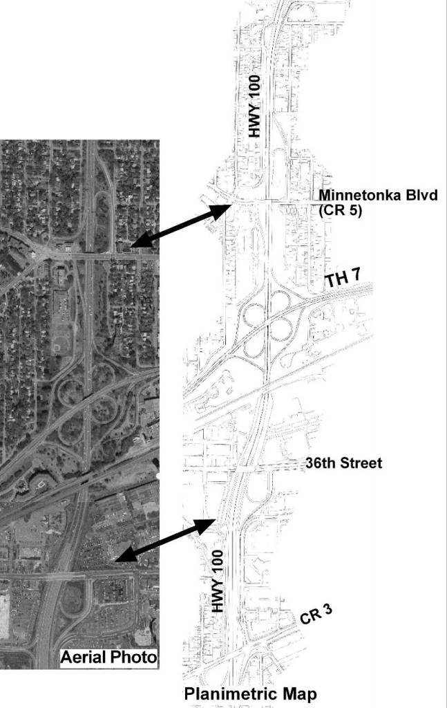
Figure 8 . Illustration. Example problem: aerial photo and planimetric map.

 

Traffic Demand Data      

Traffic volume demands were collected for the HWY 100 project using a variety of methods.  An example of a turning movement count is shown in Figure 9.  The freeway data were collected from traffic management sensors located on the freeway mainline and ramps and turning movement counts were collected manually at all locations.  A complete volume data set for both peak periods was assembled in a spreadsheet database.  The volumes were balanced reconciling differences due to counts on different days and bad detector data.

 

 

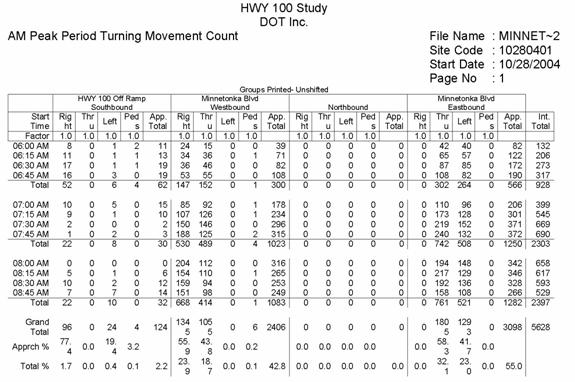
Figure 9 . Chart. Example problem: turning movement count.

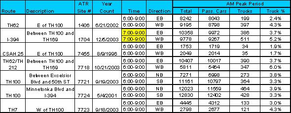
Truck Percents and Fleet Composition

Heavy truck data are collected on the system on a bi-yearly basis at several traffic data collection sites in the modeling area.  Historical count data at the relevant stations were assembled into the database as is shown in Table 7 for the a.m. peak period.

Table 7 . Example problem: heavy truck and fleet composition data.

Traffic Control Data

There are a number of traffic signals and ramp meters in the study area.  The data was gathered from three separate sources:  1) as-built traffic signal and timing plans obtained from the three operating agencies in the study area, 2) ramp metering timings and information collected from the Traffic Management Center, and 3) field observations of the traffic signal and ramp meter operations performed to confirm the as-built timing plans.

The following information was gathered from these data sources:

• Detector locations.
• Detector types (i.e., passage or presence).
• Signal phasing.
• Special phasing or sequence of operations.
• Lane geometrics and storage lane lengths.

Calibration Data

HWY 100 is a complex freeway system with closely-spaced interchanges and ramps.  Isolating a specific location that can be used to calibrate capacity was difficult.  In order to illustrate the process and to show how data can be correlated, a number of calibration samples have been assembled.  These include capacity, saturation flow rates, and freeway speeds (travel time).

Capacity

The bottleneck location to be used for calibrating capacity was not obvious.  Figure 10 shows the entire congested area for northbound HWY 100 and illustrates that the congested area for this study extends throughout the length of the reconstruction area.  Within the congested area are a number of individual bottleneck locations including a lane drop at 36th Street, and closely-spaced weaves at TH 7 and between TH 7 and Minnetonka Blvd.  This project was unusually complex with the effects of bottlenecks overlapping in such a short area.

The target capacity for calibration is shown in the hourly flow chart between Minnetonka Blvd Entrance and the 25th ½ Exit.  After the Minnetonka Blvd entrance, traffic flow picks up to a maximum hourly rate for 15 minutes of 2,654 veh/h.  This high rate is not maintained for the entire hour; therefore, the peak hour volume between 7:00 and 8:00 a.m. of 4,928 vehicles is at a rate of 2,464 veh/h per lane. 

 

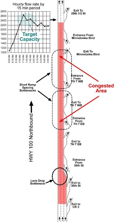
Figure 10 . Illustration. Example problem: freeway bottleneck locations.

 

Saturation Flow Rates

Saturation flow rates for one signalized intersection were checked in the field and found to match CORSIM default discharge headways.

Freeway Speeds

Speed observations were collected using the floating car technique.  The floating car was used to validate the spot speeds calculated from surveillance detectors in the pavement.  Figure 11 illustrates the data from northbound Highway 100 in the morning peak.  The simulated data will be plotted onto the same graphic.  The two different charts show that the detector data was representative of observed speeds in the field.

 

 

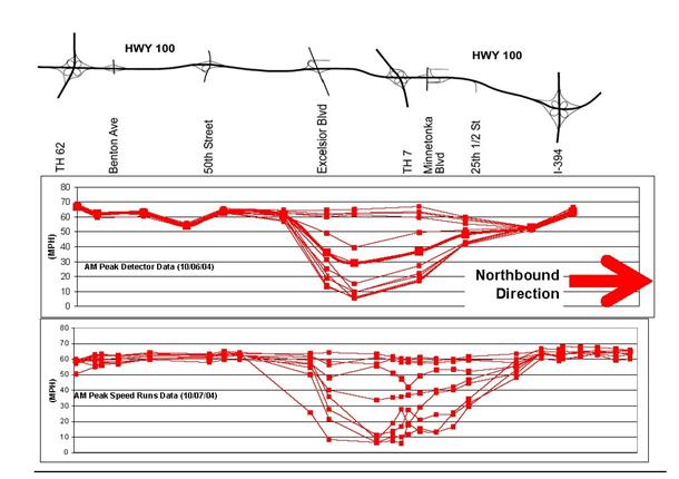
Figure 11 . Graph. Example problem: freeway travel time summary.

Data Preparation

All the data that was gathered for this project was assembled into electronic data bases.  The freeway schematic shown in Figure 12 was created in a spreadsheet and will ultimately be linked with the model results.  Figure 13 shows the example lane schematic for Minnetonka Boulevard.

 

.

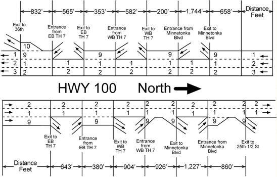
Figure 12 . Drawing. Example problem: HWY 100 lane geometry schematic.

 

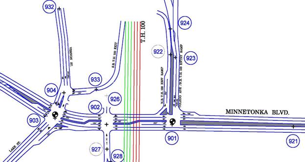
Figure 13 . Drawing. Example problem: Minnetonka Blvd. lane geometry drawing.

Field Observations

Field observations were conducted using a variety of techniques.  During travel time runs, general observations were made about congestion and hot spot locations, as well as how drivers were using the system.  In addition to observations from a driver’s perspective, observations were made from bridge overpasses and Freeway Surveillance Cameras.  Photos and video were taken to highlight significant operational issues that occurred.