Appendix C: Initialization Period

This appendix provides guidance on the estimation of the duration of the initialization period, after which the simulation has stabilized and it is then appropriate to begin gathering performance statistics.

Initialization Period, Fill Time and Equilibrium

Large networks need longer fill time for vehicles to reach their destination.  If equilibrium is not reached, a steady state is not present.  Even if the conditions that indicate that equilibrium has been reached are satisfied, a steady state may still not be present.  There are conditions where the network may report reaching equilibrium when in actuality it has not.  These conditions are discussed in this appendix.

If equilibrium is not reached or is falsely reported as being reached, the statistics that are gathered in the early portion of the simulation will not reflect conditions as they are in the real world.  The MOEs gathered during non-equilibrium periods also affect cumulative data for the entire simulation. 

Figure 67 shows a graph of the number of vehicles discharged from an internal link in an example network that has a constant volume (i.e., no variation in demand).  While the demand is constant for this network, the internal link does not reach a steady state until approximately four minutes into the simulation due to the time it takes for all portions of the network to fill up with vehicles.  It is clear from the figure that the initialization period should be at least four minutes in this example, when equilibrium has occurred on the internal links. 

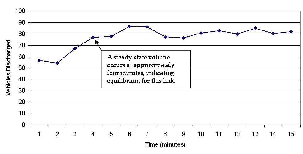
Figure 67 . Graph. Vehicles discharged from an internal link in equilibrium example.

If the specified maximum initialization time is not an integer multiple of the time interval specified, the program will round it down to the nearest integer multiple of the time interval.  The algorithm to test for equilibrium requires the initialization time to be at least three time intervals.  If the specified initialization time is less than three time intervals, the program will automatically increase initialization time to three time intervals.

The analyst selects the initialization options in TRAFED on the Network/Properties dialog on the Run Control Page.  These options are discussed below.

Use initialization period

The analyst may want to turn off the initialization period to view how the network fills or to collect statistics during the initialization period for research purposes.  This is a very useful debugging tool and also a valuable teaching tool.

Maximum initialization prior to simulation

This is the amount of time that CORSIM will use as its maximum initialization period.  CORSIM can determine that it has reached equilibrium prior to this time and start the simulation and collection of statistics.  CORSIM will not run longer than this time in the initialization period.  A message will be displayed to indicate whether or not equilibrium has been reached.  A rule of thumb is to set this time to the travel time for the longest realistic path through the network.

Stop if initialization does not reach equilibrium

If the maximum initialization period time has been reached and equilibrium has not been achieved, then the simulation will either start collection statistics or stop depending on this setting.  Stopping the run will prevent data for that run from being used in the statistical output.

Force maximum initialization time

CORSIM may falsely determine that it has reached equilibrium.  The analyst can force CORSIM to stay in the initialization period until the maximum time has expired.  For example, a very large network may have a number of vehicles entering at the extreme upstream entry point and on-ramps near the downstream exit point.  If the number of vehicles entering and exiting are similar, CORSIM may determine that equilibrium has been reached well before the entering vehicles can traverse the length of the network.

The initialization period runs until either equilibrium is reached or the maximum time allowed for initialization is reached.  When the time allowed has been reached and equilibrium has not been reached the simulation will begin unless the user specified that the simulation should abort in that case.  When equilibrium is reached during the initialization period, initialization will terminate unless the user specified that initialization should run for the entire time allowed.

Equilibrium is determined by comparing the number of vehicles in the network on consecutive time intervals.  If the difference between the current interval and the previous interval is less than eight percent and the difference between the previous interval and the one before it was less than 12 percent, CORSIM determines that equilibrium has been reached.  If those conditions have not been met, but the difference between the current interval and the previous interval is less than six percent, CORSIM determines that equilibrium has been reached.

The example network in Figure 68 would reach equilibrium prior to the 360-second point.  It would reach it at 300 seconds because the previous interval (240 seconds) percent was less than 12 and the current percent is less than 8.  If the user requested the full time to reach equilibrium, the initialization would continue to the 420-second point.  If force maximum initialization time is not requested, the initialization would end and the simulation would reset the clock to zero and start collecting statistics.  Even if the above were not satisfied, the network would have been considered in equilibrium at the 360 second mark because the 3 percent difference (6.6 – 3 = 3.6%) is less than 6 percent difference.

 

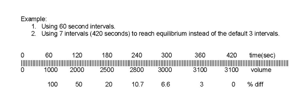
Figure 68 . Illustration. Reaching equilibrium.

 

This process does have some flaws.  Specifying small (one second) time intervals terminates the initialization period too early because the volume does not increase enough between periods.  Very large networks with high volumes do not allow vehicles to reach the center of the network before equilibrium is satisfied because the percentage of volume does not change enough.  That is why the ability to force the full initialization period to occur was added to CORSIM.

When modeling a network that includes long distances, where travel time may be significant, the travel time must be taken into account when setting up the simulation.  Initialization (fill time) uses the conditions at the beginning of the simulation to fill the network of roadways.  Use caution to use input data that will reflect the true conditions at locations well downstream.  In order to accurately model the conditions during a period of interest, it may be necessary to start modeling the network with data for the time prior to the start of the analysis.

For example, when modeling a 24.1 km (15 mi) stretch of freeway with three on-ramps, take into account the time it takes to travel 24.1 km (15 mi).  If the traffic is averaging 96.6 km/h (60 mi/h), then it will take 15 minutes to travel from the entry point to the end of the freeway.  If the analysis period starts at 7:30 a.m. and lasts until 8:00 a.m., the actual number of vehicles that come onto the freeway from 7:30 to 7:45 a.m. and from 7:45 to 8:00 a.m. could be input.  However, using these counts as the starting counts for the analysis, a 15-minute initialization period (travel time through the network) will use the 7:30 counts to fill the whole network.  In actuality, the vehicles departing the freeway crossed the entry point (data station or tube counter) at approximately 7:15 a.m.  If the volume of traffic between 7:15 and 7:30 a.m. is significantly different than it is from 7:30 to 7:45 a.m., then traffic conditions downstream will be significantly different.

As mentioned previously, the analysis period chosen should begin before the onset of congestion and end after the dissipation of all congestion to ensure that all queued demand is eventually included in the analysis.  Further, this discussion on the initialization period shows that beginning the analysis period when demand is increasing sharply from an uncongested to congested state can cause the demand in the first analysis period to be unrepresentative of the actual demand.  As a result, the timing of the first analysis period is an important consideration, especially when demand is increasing sharply, and simulating an additional time period before the actual analysis period would better capture the true demand under these circumstances.