Appendix A: Introduction to CORSIM Theory
This appendix provides an introduction to the fundamentals of CORSIM model theory.
CORSIM has a long history reaching back to the 1970s and mainframe computers. Many fixes, improvements, and enhancements have been made since the original coding but the basic theory of CORSIM still retains its roots. In 1994 two separate programs, one for modeling surface streets (NETSIM) and one for modeling freeways (FRESIM), were combined to form the CORSIM program. CORSIM can model both uninterrupted and interrupted types of facilities. Each facility is modeled in a separate “subnetwork”.
“Uninterrupted flow facilities have no fixed elements, such as traffic signals, that may interrupt the traffic flow. Traffic flow is a result of the interactions among vehicles in the traffic stream and between vehicles and the geometric and environmental characteristics of the roadway.” (3)
Uninterrupted flow facilities in CORSIM are represented by freeways. They are modeled internally in CORSIM using code that came from FRESIM (abbreviated for FREeway SIMulation). FRESIM was the successor to FHWA’s freeway simulation program called INTRAS, which was developed in the late 1970s.(21) Its purpose was to assess the effectiveness of freeway control and management strategies. INTRAS was originally developed to work on a mainframe computer, while FRESIM was developed to operate on a microcomputer.
“Interrupted flow facilities have fixed elements that may interrupt the traffic flow. Such elements include traffic signals, stop signs, and other types of controls. These devices cause traffic to stop periodically (or slow significantly), irrespective of how much traffic exits.” (3)
Interrupted flow facilities in CORSIM are represented by surface streets. They are modeled internally in CORSIM using code that came from NETSIM (abbreviated for NETwork SIMulation). NETSIM was originally developed as the “Urban Traffic Control System” (UTCS-1) in the early 1970s. It was created for FHWA’s test bed in Washington, DC.(8) The program evolved under the direction of the FHWA and was later named NETSIM.
The physical environment is represented as a network composed of nodes and unidirectional links. The links generally represent urban streets or freeway sections, and the nodes generally represent urban intersections or points at which a property changes (such as a change in grade or free-flow speed). In a corridor simulation with both surface streets and freeways, each type of facility is referred to as a subnetwork.(1) Vehicles in CORSIM travel from one subnetwork to another subnetwork on a second-by-second basis.
CORSIM applies time step simulation to model traffic operations. This is called a microscopic model, wherein the behavior of every vehicle is represented at each time step. Other types of models include macroscopic and mesoscopic. A microscopic simulation, such as CORSIM, models individual vehicle movements based on car-following and lane-changing theories on a second-by-second basis for the purpose of assessing the traffic performance of highway and street systems. In a macroscopic model, platoons of vehicles are moved on a section-by-section basis over short time periods rather than by tracking individual vehicles every second. Macroscopic models do not have the ability to analyze transportation movements in as much detail as microscopic models and therefore have fewer computer requirements. A mesoscopic model combines the properties of both microscopic and macroscopic models. The vehicle movements are based on local prevailing speeds, consistent with established macroscopic speed-density relationships.
CORSIM is a stochastic simulation model, which means that it incorporates random processes to model complex driver, vehicle, and traffic system behaviors and interactions. Stochastic simulation models produce output that is itself random. On the other hand, a deterministic model produces output that is “determined” once the set of input quantities and relationships in the model have been specified. The Highway Capacity Model (HCM) is an example of a deterministic model.
Note that a random process is directly related to an observed behavior. For example, at a particular intersection it can be observed that twenty percent of the vehicles turn left. In CORSIM, a random number is drawn each time a vehicle makes a turn decision. If the random draw produces a number that is twenty or below, the vehicle will be assigned a left turn. This may produce three vehicles that turn left in succession or it may not produce a left turning vehicle in 100 draws. However, over the course of a large number of vehicle decisions, twenty percent of the vehicles will end up turning left. In contrast, if the twenty percent was used directly without modeling a random process, every fifth vehicle would turn left. This would produce the correct percentage of vehicles turning left, but would not represent the behavior observed in the real world.
Because the output of a stochastic model is random, each run of a stochastic simulation model produces only estimates of a model’s true characteristics for a particular set of input parameters. Thus, relying on the MOEs generated from a single run of CORSIM may be misleading. To produce meaningful MOEs, several independent runs of the model will be required for each set of input parameters to be studied. For example, a single run may result in three very conservative drivers driving side-by-side on a three-lane roadway, blocking more aggressive drivers behind them. The resulting MOEs would reflect a lower average speed and higher travel time than has been observed in the real world, although it is possible that this scenario could happen in the real world given enough observations. To gain a better understanding of network performance, the network should be simulated several times using different sets of random number seeds (to produce a different series of random draws). The resulting distribution of MOEs should then be an accurate representation of the network performance.
CORSIM uses three random number seeds during each simulation run to decide many processes. One random number seed is used in generating vehicle entry headways, one is used to determine surface street routing, and one is used to determine time dependent stochastic processes like time and location of parking and short term events. When a vehicle uses a random number it stores a new random number seed to be used the next time a random number is required. This sequence of random number seeds is repeatable.
The first random number seed is used to generate vehicle entry headways. Stochastic vehicle entry headways can be generated from a normal distribution, negative exponential distribution, or Erlang distribution (see appendix E for more detail on vehicle entry headway distributions). By default, CORSIM emits vehicles from entry links and source links at a constant rate, derived from the input volume. The user can vary the vehicle generation by selecting a distribution of the entry times instead of a constant rate and change this seed between runs to produce variation in the times that vehicles are scheduled to enter the simulated roadways. Note that the total number of vehicles due to be emitted will remain the same between runs even though the time between individual vehicle emissions will vary.
A second random number seed is used in generating vehicles for the surface street traffic stream. Decisions such as the routing pattern of each vehicle and the characteristics of each driver/vehicle combination are generated from this base seed. The user should keep this entry constant during multiple runs if he/she wants to obtain identical traffic movements. A series of runs with different values for this random number would illustrate the variance in the traffic performance measures of effectiveness that are due to variations in traffic patterns.
The third random number seed is used by CORSIM for all stochastic processes other than vehicle headway generation and traffic stream generation. It is used in all time-dependent stochastic decision-making processes (e.g., accepting available gaps for turns, determining location and duration of lane blockages, calculating pedestrian inter-arrival times, and determining lane change gap acceptance risk). The user should vary this entry during multiple runs to obtain different traffic environments. By changing this random number seed and keeping the traffic random number seed constant, the user can simulate with traffic streams exhibiting identical routing and driver/vehicle characteristics, but in a stochastically-derived traffic environment.
A more detailed description of random numbers in CORSIM is given in appendix D.
Each vehicle is identified by fleet (auto, carpool, truck, or bus) and by type. Up to sixteen different types of vehicles (with different operating and performance characteristics) can be specified, thus defining the four vehicle fleets. Furthermore, a "driver behavioral characteristic" is assigned to each vehicle. Each vehicle is assigned one of ten different “driver types” that increase in aggressiveness from 1 to 10. Its kinematic properties (speed and acceleration) as well as its status (queued or moving) are determined. Turn movements are assigned stochastically, as are desired free-flow speeds, queue discharge headways, and other behavioral attributes. As a result, each vehicle's position and behavior can be simulated in a manner reflecting real-world processes.
Vehicles are allocated to the network via an imaginary link called an entry link. The vehicle characteristics (such as type of vehicle, driver type, desired lane, and desired speed) are stochastically assigned. The vehicle will enter the network at user assigned volumes at intervals stochastically determined by the user’s preferred method of emission.
In general, a vehicle that is not influenced by other vehicles or network objects will attempt to increase its acceleration to the maximum possible value in an effort to attain a desired free-flow speed. When the desired free-flow speed has been attained no more acceleration is allowed. Each of the ten driver types will have a desired free-flow speed on a particular link that is equal to the facility free-flow speed adjusted by a multiplier unique to the driver type. The free-flow speed of the facility is defined as the speed in free flowing conditions such as a low volume condition.
The car-following logic assumes that a follower vehicle will maintain a desired headway between itself and its leader. The distance between the vehicle and its leader will depend on the speed the vehicle is traveling. For example, if a vehicle is traveling at a speed of 27.4 meters per second (m/s) (90 feet per second (ft/s)), and has a desired headway of one second, it will try to maintain a distance of 27.4 m (90 ft) from its leader. Each of the ten driver types has a unique, desired headway. If the current distance is not sufficient to maintain the desired headway, the vehicle will decelerate in an effort to attain the desired headway. If the distance is larger than the desired headway the vehicle will attempt to accelerate to achieve the desired headway unless it is at its desired free-flow speed.
The behavior of a lead vehicle is also dependent on the upcoming network characteristics (e.g., changes in lane configuration, turning movements, control, blockages, etc.). The vehicle will scan the upcoming network objects and attempt to adjust its speed or lane in order to react to the objects.
A vehicle that must make a lane change due to a lane drop, exit, turn, or blockage will make a “mandatory” lane change. A mandatory lane change is the most stringent of the types of lane changes. Vehicles will accept a higher risk (deceleration) as the vehicle approaches the network object requiring the lane change. A vehicle that is traveling slower than its desired speed may find it advantageous to change lanes to achieve a higher speed. This type of lane change is referred to as a “discretionary” lane change.
CORSIM accumulates different types of data every time step (i.e., every second). These “raw” data, such as travel time and distance traveled, are gathered as the vehicles move and interact with other vehicles and traffic control objects. At the end of each user specified time interval the accumulated “raw” data is used to report MOEs and produce other MOEs. For example, the distance traveled is divided by the travel time to produce an average speed.
Vehicle Mix
CORSIM only allows four different fleets (Passenger Car, Truck, Bus, and Carpool) and defaults to nine vehicle types. By default, only the Passenger Car Fleet is used. The vehicle mix attributed to Trucks and Carpools must be input by the analyst or they will not be used. If Trucks and Carpools are requested they will default to the percent of fleet shown in Table 20. Prior to combining NETSIM and FRESIM to form CORSIM, each subnetwork had its own vehicle type identifiers. In the table, both the NETSIM (N) and FRESIM (F) identification numbers and the default percentage of fleet for each vehicle type are listed.
Table 20 . Default CORSIM vehicle specifications.
|
Fleet | Vehicle ID and Type |
Perform. Index |
Length |
Occupants |
Default % of |
|---|---|---|---|---|---|
PASSENGER |
2(F) 1(N) = High performance |
2 |
16 |
1.3 |
75(F) 75(N) |
TRUCK |
3(F) 2(N) = Single unit |
3 |
35 |
1.2 |
31(F) 100(N) |
BUS |
7(F) 4(N) = Conventional |
7 |
40 |
25.0 |
100(F) 100(N) |
CARPOOL |
9(F) 3(N) = High performance |
9 |
16 |
2.5 |
75(F) 100(N) |
Notes: (F) = FRESIM, (N) = NETSIM.
Each vehicle type must belong to one or more of the fleets. The percentage of a fleet for all vehicle types that make up the fleet must add up to 100 percent. For example, a 10.7 m (35 ft) single unit truck could make up a percentage of the Truck fleet and also make up a portion of the Bus Fleet when modeling a second, shorter bus type. However, the Conventional bus type percent of the Bus fleet would need to be reduced to make the total Bus fleet add up to 100 percent. Surface streets and freeways can have their own percentage of the vehicle type within the fleet.
The table also shows the default performance index, default length, and default average number of occupants for each vehicle type. The length specifies the bumper-to-bumper length of a vehicle type. The occupants (load factor) are used to accumulate and calculate MOE related to numbers of people.
Performance Index
CORSIM maintains tabulated data for maximum acceleration, fuel consumption, and environmental emissions as well as for the effect of grade on acceleration and fuel consumption. These tables are referenced by vehicle speed and (for environmental emissions and fuel consumption only) acceleration. CORSIM contains seven different tables for each of these data types. The seven tables correspond to the seven groups of vehicle performance. The seven groups are referenced by the Performance Index. The analyst can specify which of the seven tables best describes the defined vehicle performance. The default tables should be used unless there is adequate support to deviate from the defaults.
Acceleration Tables
CORSIM allows the analyst to modify any or all of the tabulated data that define maximum acceleration, grade correction factor for maximum acceleration, and grade correction factor for fuel consumption. The data are input for speeds in 10 ft/s speed intervals. Values in between those entered are computed internally by the CORSIM model via linear interpolation.
Figure 65 shows a graph of the default maximum acceleration in feet per second squared for each speed in feet per second for the seven different performance indexes. High performance vehicles use performance index two while heavy trucks use performance indexes five and six.
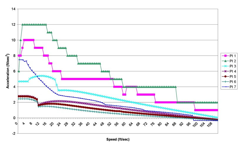
Figure 65 . Graph. Maximum acceleration versus speed by performance index.
Vehicle Fuel Data and Vehicle Emissions
CORSIM allows the user to modify any or all of the parts of internal data tables defining fuel consumption and pollutant emission rates. The tables express these rates as a function of acceleration, given the vehicle performance index and vehicle speed. Figure 66 shows the default fuel consumption rates versus the speed at different acceleration rates. Similar tables exist for different types of vehicle emissions.
This data is difficult to collect and calibrate and has not been updated within CORSIM in many years. It is recommended to use this data for comparison analysis only. Do not use this data as an absolute indication of the capabilities of today’s vehicles. For example, it may not be valid to report that 200 fewer grams of hydrocarbons were emitted using a certain alternative. It may be more proper to report a 10 percent decrease in emissions with a certain alternative.
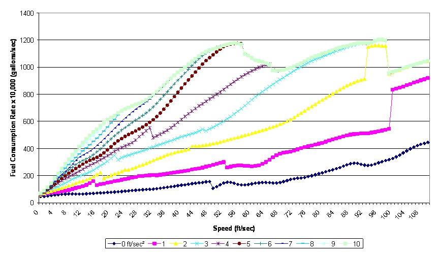
Figure 66. Graph. Fuel consumption for different acceleration rates for performance index 1.
Fleet Type
The need to assign each vehicle type to one or more fleet components reflects the fact that several considerations are based upon the identification of fleet components. Each vehicle processed by the model is identified by type and fleet component. For example, the analyst can reserve lanes for buses and carpools, specify data so that certain streets are reserved for buses, and specify the percentage of trucks and carpool vehicles on each entry link. Bus vehicles are assigned routes and stations. A carpool fleet can include several vehicle types (such as automobiles and minibuses), or a bus fleet can include several different types of buses with different performance characteristics because a vehicle type can be part of one or more fleet components
Vehicle Types
CORSIM allows the user to create or modify up to 16 different vehicle types. Each vehicle must be part of one or more of the vehicle fleets. 100 percent of each vehicle type must be allocated to the different fleets. Each vehicle type must use one of the seven existing or modified vehicle performance indexes. These are used to determine the vehicles acceleration, emissions, and fuel usage. Each vehicle type may have its own characteristics.
Freeway Vehicle Parameters
In addition to the vehicle parameters listed above, freeway vehicles have some separate user-modifiable parameters including Jerk Factor and Maximum Deceleration Rate.
Jerk Factor
The jerk factor (rate of change of acceleration) value is the maximum change allowed in the value of acceleration from one time step to the next for a vehicle type. It is input in tenths of feet per second cubed.
Maximum Deceleration Rate
The maximum deceleration rate is the maximum deceleration on level grade and dry pavement for a vehicle type. It is used in car-following and lane-changing.
Surface Street Vehicle Parameters
In addition to the vehicle parameters listed above, surface street vehicles have an additional user-modifiable parameter called the Headway Factor. The Headway Factor defines a multiplicative factor applied to the mean discharge headway that was assigned on a link-specific basis. This factor reflects the difference in queue discharge headway between a “typical” passenger car and this vehicle type.