
U.S. Department of Transportation
Federal Highway Administration
III. Signal Timing Tool Box
When most Traffic Engineers consider signal timing, the first thought invariably involves the computerized optimization models. Issues like which model is best, and what are the minimum data required to use the model, are typical topics. Over the years, much research effort has been invested in developing these models, and of all of the steps in the signal timing process, the evolution of the signal timing optimization models is the most highly developed.
When one mentions the word, “model,” most automatically think of a computer model. But it is important to recognize that a model can also be a manual model.
The following sections provide a description of various manual and automated techniques that can be used to develop timing plans. These techniques can be used to estimate parameters directly, or to estimate various inputs to signal timing optimization computer programs that will be used to generate timing plans. The basic concept underlying the approach to minimizing timing plan development cost is to identify those parts of the process when resources should be directed to achieve the best benefit, and conversely, identify areas where parameters can be approximated.
Data Collection Tools
Regardless of what computer model or manual process the Engineer chooses to use to develop the timing plans, all require network descriptive information and turning movement data. All signal optimization and simulation models, even manual signal timing procedures, require a physical description of the network. This description includes distance between intersections (link length); the number and type of lanes; lane width, length, and grade; permitted traffic movements from each lane; and the traffic signal phase that services each flow. Building a network from scratch is a significant undertaking. But once the network is defined, in general, only traffic demand and signal timing parameters have to be updated to test a new scenario. The tools related to data collection are provided below.
Intersection Categorization
The intersection may be categorized as either Primary or Secondary. The primary intersections are the ones that have the highest demand to capacity ratio and will, therefore, require the longest cycles. These intersections are usually well known to the Traffic Engineer. They are the intersection of two arterials, the intersections with the worst accident experience, the intersections that service the major shopping centers, and the intersections that generate the most complaints. The secondary intersections are the ones that generally serve the adjacent residential areas and local commercial areas. They are usually characterized by heavy demand on the two major approaches and much less demand on the cross-street approaches.
The purpose of assigning intersections to one of these two categories is to reduce the locations where traffic counts are required. The primary intersections require turning movement traffic counts—there is simply no other way to measure demand. However, the secondary intersections usually have side street demand that can be met with phase minimum green times (usually between 8 and 15 seconds with lower values if presence detection is provided near the stop bar). The strategy, therefore, is to concentrate the counting resources at the locations where there is no substitute, and to use minimum green times for the minor phases at secondary intersections.
This categorization is important because more and costly data is needed for the Primary intersections than for the Secondary intersections. Many of the timing parameters for the Secondary intersections will be estimated rather than calculated, and therefore, are subject to larger errors.
This characterization is very subjective, and to a great extent, the categorization depends on the budget available for signal timing. If the budget is small, fewer intersections would be considered Primary; if the budget is moderate, more intersections on the cusp would be considered primary.
Short-Count Method
Regardless of whether manual or computerized signal timing models are planned to be used, there is a need for turning movement count input to the process. The turning movement count is the single most costly element in the signal timing process, and therefore, is generally the most significant impediment to overcome. One way to reduce the expense of data collection is to reduce the time required to collect the data. Many traffic engineers use “short counts” to meet this objective. Short counts are normal turning movement counts that are conducted over periods that are less than normal.
The basic concept of the short count is to take a sample of the turning movements during the period of interest and to expand the short period to reflect an estimate of the demand during the entire period. Fifteen-minute samples are typical and they are expanded to hourly flow rates for use in the various signal timing procedures. One method of developing these counts, the Maximum Likehood model, was defined by Maher in 1984.3
If the agency does not have a procedure in place for conducting short counts, the following is suggested:
Determine the beginning and ending time of the period for which the count is intended to represent
Within this time window identified above, start a stop watch when the yellow ends for the through movement on the approach being observed
Record the number of vehicles turning left, through, and right during the cycle measured from the end of yellow to the end of yellow during each cycle
Continue recording the counts at the end of each cycle until at least 15 minutes have elapsed and at least eight cycles are recorded
For the last cycle, add the number of vehicles in queue (if any) to the count for the last cycle
Record the time on the stop watch (10 minutes or more)
Convert the counts to an hourly flow rate for each movement.
Estimated Turning Movements
When turning movement counts are not available, it is sometimes possible to estimate the turning movements when approach and departure volumes are known and some information is available concerning the intersection flows.
The National Cooperative Highway Research Program (NCHRP) developed techniques for estimating traffic demand and turning movements. These techniques are described in NCHRP 255, “Highway Traffic Data for Urbanized Area Project Planning and Design.” One of the procedures described in this document derives turning movements using an iterative approach, which alternately balances the inflows and outflows until the results converge (up to a user-specified maximum number of row and column iterations).
Dowling Associates, Inc., a traffic engineering and transportation planning consulting firm based in Oakland, California developed a program, TurnsW, that can be used to estimate turning volumes given approach and departure volumes. This program is available from http://www.dowlinginc.com/ (under downloads). The user may “lock in” pre-determined volumes for one or more of the estimated turning movements. The program will then compute the remaining turning volumes based upon these restrictions.
Signal Grouping
To state the obvious, all signals that are synchronized together must operate on the same cycle length or a multiple of that cycle length. Since it is unlikely that all primary intersections will have the same cycle length requirements, some method must be used to arrive at a common cycle length. Engineering judgment usually prevails in this area. For example, if there are three intersections requiring 75-, 80-, and 110-second cycles, the 110-second cycle must be used. However if the results were 80, 80, and 85, then an 80-second cycle may be appropriate. In general, the longest cycle length would be used.
Another important point to make regarding the grouping of intersections is that the need to group the intersections is based on traffic demand. Since it is likely that traffic demand is different during different times of the day, it is reasonable to expect that different groupings of intersections may be appropriate during different times of the day. In practice, this may mean, for example, that an intersection is associated with a group and operates with the common group cycle length during a peak period, but operates as an isolated intersection during other time periods. It is important to recognize that intersection groupings are a function of traffic demand, and signal groupings are not a static condition.
Coupling Index
The Coupling Index is a simple methodology to determine the potential benefit of coordinating the operation of two signalized intersections. The theory is based on Newton’s law of gravitation, which states that the attraction between two bodies is proportional to the size of the two bodies (traffic volume) and inversely proportional to the distance squared. In equation form, the Coupling Index is:
CI = V / D2
Where:
CI = Coupling Index
V = Two-way total traffic volume peak hour / (1000 vph)
D = Distance between signals (miles)
There are several variations of this approach. The “Linking Factor” as used by Computran in Winston Salem, NC, and the “Offset Benefit” as described in NCHRP Report 3-18 (3) are two examples of different similar techniques that have been used to determine signal group boundaries.
A recent review and analysis of these grouping methods by Hook and Albers concluded that there is no absolute best method to use for determining where system breaks should occur.4 The authors further concluded that each method gives about the same result and the simpler methods are just as valid as the complicated methods. In general, they suggested that the following criteria be used:
Group all intersections that are within 2,500 feet of one another.
Use all links that are 5,000 feet or more in length as boundary links.
Calculate the Coupling Index for all links between 2,500 feet and 5,000 feet in length and link all intersections that have a value greater than 50, consider linking intersections that have a value of 1 to 50, and do not link intersections that have a value of less than 1.
The following process is suggested for use with any of the Index procedures. The first step is to determine which sections of roadways are to be analyzed. These links are then drawn on a map, which may be distorted to provide space to display information related to each link.
Various traffic data can be superimposed over the roadway network to determine applicable traffic volumes for the particular segment being registered. Some links may not have any corresponding traffic data. In which case, the segment is still registered, but with a zero value given for the traffic volume, which in turn results in a Coupling Index of zero.
The next step is to calculate the indices for all of the registered links. The final step is to identify signal groups by linking together intersections with high index values and identifying group boundaries using links with low index values.Major Traffic Flows
Another factor that should be considered when considering intersection groupings is traffic-flow demand paths. With an arterial, this issue is moot, but with a grid network, it can be crucial. With the grid pattern shown in top chart in Figure 3, the horizontal dashed line shows a likely group boundary. However, when a major traffic-flow pattern does a dogleg, as shown in the bottom chart of Figure 3, then a different group boundary may be appropriate. This characteristic will probably manifest itself in the index, but when the signal engineer must make decisions based on sparse data, then knowledge of traffic-flow patterns can be a useful discriminator to identify group boundaries.
Coordinatability Factor
There is one additional technique than can be employed by those that use the computer program, Synchro. Synchro has an internal methodology to calculate a “coordinatability factor.” This factor considers travel time, volume, distance, vehicle platoons, vehicle queuing, and natural cycle lengths. The coordinatability factor is similar to the “strength of attraction,” but also considers the natural cycle length and vehicle queuing. The natural cycle length is defined as the cycle at which the intersection would run in an isolated mode or the minimum delay cycle length. The potential for vehicle queues exceeding the available storage is also considered in determining the desirability of coordination.
Number of Timing Plans
The “rule of thumb” for the number of signal timing plans is that each group requires a minimum of four plans: morning peak plan, average day plan, afternoon peak plan, and evening plan. But each signal group is unique, and each group has unique demands. For example, an arterial that provides access to a regional shopping center may experience major demands on Saturday. Other examples abound of locations that require different timing plans to meet demands by other major traffic generators, such as amusement parks, recreational demands, and other non-work-related trips.
One analytical method that can be used to estimate the need for a special timing plan is to plot the arterial traffic by direction and by time of day. The plot of the sum of both directions provides an indication when cycle length changes may be required. Longer cycles are typically required to service heavier volumes. The ratio of one direction to the total traffic by time of day provides a good indication when offset changes may be required. The number of plans required and the time during which they will be used is needed to schedule the site surveys described in the next section. Analysis of the traffic demands at individual intersections will indicate when split changes are required.
Cycle Length Issues
As noted above, having a common cycle length is fundamental to coordinated signal operation. The cycle length must be evaluated from two different perspectives: individual intersection and the group cycle length.
For the individual intersection, the recommended approach is to focus on the one or two major intersections in the group—the intersections with the highest demand because these are the ones that will set the minimum cycle length limits. When evaluating cycle lengths, it is important to verify that the pedestrian timing is sufficient to allow pedestrians to cross the street. When the pedestrian timing is known, say 7 seconds to Walk, 10 seconds for Pedestrian Clearance, and 3 seconds for yellow change, and the vehicle phase is to be allocated at least 25 percent of the cycle, then the minimum cycle length that can meet both constraints is 20 seconds divided by 25 percent, or 80 seconds (assuming two critical phases).
In general, the intersection in the group that requires the longest cycle length will set the group cycle length. The cycle length and splits can be determined by using either Webster’s equation or the Greenshields-Poisson Method. Both of these methods are explained below. In general, for a given demand condition, there is a cycle length that will provide the optimum two-way progression. This cycle length is a function of the speed of the traffic on the links between intersections and the link distance between intersections. This cycle length is called the “Resonant Cycle,” and is explained further below.
Webster’s Equation
One approach to determining cycle lengths for an isolated pre-timed location is based on Webster's equation for minimum delay cycle lengths. The equation is as follows:
Cycle Length = (1.5 * L + 5) / (1.0 -Yi)
Where:
L = The lost time per cycle in seconds
Yi = Sum of the degree of saturation for all critical phases 5
This method was developed by F.V. Webster of England's Road Research Laboratory in the 1960s. The research supporting this equation is based on measuring delay at a large number of intersections with different geometric designs and cycle lengths. These observations yielded the equation that is used today. It is important to recognize that this work assumed random arrivals and fixed-time operation—two conditions that can rarely be met in the United States. Notice that the equation becomes unstable at high levels of saturation and should not be used at locations where demand approaches capacity. Nevertheless, this technique provides a starting point when developing signal timings. To use this equation:
Estimate the lost time per cycle by multiplying the number of critical phases per cycle (2, 3, or 4) by 5 seconds (estimated yellow change plus red clearance time) to determine the “L” factor. L will have a value of 10, 15, or 20 and the numerator will equate to 20, 27.5, or 35 seconds.
Estimate the degree of saturation for each critical phase by dividing the demand by the saturation flow (normally 1900 vehicles per hour per lane).
Sum the degree of saturation for each critical phase and subtract the sum from 1.0. This is the denominator.
To obtain the cycle length, round the division to the next highest 5 seconds.
Greenshields-Poisson Method
This approach to signal timing is statistically-based and makes several assumptions about the behavior of traffic. It uses the Poisson distribution to describe the arrival patterns of vehicles at an intersection. This distribution assumes that the vehicles travel randomly. This assumption is frequently a problem in urban areas, but like other methods, it can provide a good starting point to develop signal settings.
While the Poisson distribution is used to estimate the arrivals, the time required for the approach discharge is based on work done by B. D. Greenshields in 1947. Surprisingly, this work has held up well during the intervening 50 years. Like Webster, Greenshields founded his work on many observations of traffic performance. The results of these studies are summed in the equation:
Phase Time = 3.8 + 2.1 * n
Where:
Phase Time is the required duration to service the queue
n is the number of vehicles in queue in the critical lane6The basic procedure is iterative and uses the following steps:
Assume a cycle length. For two critical phases, we suggest 60 seconds, for three critical phases, we suggest 75 seconds, and for four critical phases, we suggest 100 seconds.
a. Calculate the number of cycles per hour by dividing 3,600 (seconds per hour) by the assumed cycle length.For each critical phase, divide the demand volume by the number of lanes and by the number of cycles per hour to determine the mean arrival rate per lane.
Use the Poisson distribution (Table 1) to convert the Mean Arrival Rate to the Maximum Expected Arrivals at the 95 percentile level.
Convert this Maximum Expected Arrivals to time required using Greenshields equation.
Add the time required for each critical phase plus the clearance and change time required (nominally 5 seconds) for each critical phase. If the sum is more than 5 seconds less than the assumed cycle, repeat the steps starting with the new (shorter) cycle length. If the sum is greater than the assumed cycle length by more than 5 seconds, repeat the steps but use the 90th or 85th percentile Maximum Expected Arrivals. If the calculations using the 85th percentile arrivals indicate a cycle length greater than 80 seconds for two-phase operation, 100 seconds for three critical phases, and 120 seconds for four critical phases, then the volumes may be too high to use this method.
Table 1 Poisson Distribution.
| Mean Arrival Rate | 85 Percentile | 90 Percentile | 95 Percentile |
|---|---|---|---|
| 1 | 3 | 3 | 3 |
| 2 | 4 | 4 | 5 |
| 3 | 5 | 6 | 7 |
| 4 | 7 | 7 | 8 |
| 5 | 8 | 8 | 9 |
| 6 | 9 | 10 | 11 |
| 7 | 10 | 11 | 12 |
| 8 | 11 | 12 | 13 |
| 9 | 13 | 13 | 15 |
| 10 | 14 | 15 | 16 |
| 11 | 16 | 16 | 17 |
| 12 | 16 | 17 | 18 |
| 13 | 17 | 18 | 20 |
| 14 | 18 | 19 | 21 |
| 15 | 19 | 20 | 22 |
| 16 | 21 | 22 | 23 |
| 17 | 22 | 23 | 24 |
| 18 | 23 | 24 | 26 |
| 19 | 24 | 25 | 27 |
| 20 | 25 | 26 | 28 |
The Greenshields-Poisson Method is best suited to lower volume intersections. When the critical lane volume exceeds 400 vph then the basic assumption of random arrivals (no vehicle interactions) is probably not valid. Even within this range, care must be exercised. The method is designed to accommodate more vehicles than is expected on average; but some percentage of the time, 5 to 15 percent, the demand will exceed the time allocated and not all arrivals will be served. Care should be used to not apply this method at congested locations as the process will suggest unrealistically long cycle lengths which will result in high delay and long queues.
Cycle Length
When the traffic demand is balanced in both directions on the arterial, and when the distance between the intersections is approximately equal, then it is possible to obtain good progression in both directions by adjusting the cycle length using the following formulas:
(1) Cycle = 2 * Distance / Speed (1)
(2) Cycle = 4 * Distance / Speed (2)
(3) Cycle = 6 * Distance / Speed (3)
Where:
Cycle is the cycle length in seconds
Distance is the link length in feet
Speed is the average link speed in feet per second.These equations define resonant cycle lengths for this signal group.7 Notice that the only real-time variable in the equations is traffic speed, which is actually used to estimate link travel time. This implies that different cycle lengths would be appropriate when there is a significant change in the link speed. It is typical for link speeds to be slower during the peak periods. This implies that it may be appropriate to use a longer cycle length during peak periods.
Once an appropriate cycle length is selected using one of the three formulas noted above, the offsets can be identified as follows:
Formula (1)—The offset of an intersection at one end of the arterial is set to an arbitrary value—many engineers use 0 seconds. The offset at the next intersection is set to the sum of the value of the offset at the first intersection plus 50 percent of the cycle. For example, if the offset of the first intersection is 0 and the cycle length is 100 seconds, then the offset of the second intersection is 50 seconds. The offset of the third intersection and all other odd-numbered intersections is the same as the offset at the first intersection, 0 seconds in the example. The offset at the fourth intersection and all other even-numbered intersections is the same as the offset at the second intersection, 50 seconds in the example. This method of setting signal timing is called a Single Alternate, and is the most desirable because it provides the maximum bandwidth in both directions.
Formula (2)—The offset of two intersections at one end of the arterial are set to an arbitrary value—0 seconds, for example. The offset at the next two intersections are set to the sum of the value of the offset at the first intersection plus 50 percent of the cycle. For example, if the offset of the first and second intersection is 0 and the cycle length is 100 seconds, then the offset of the third and fourth intersections is 50 seconds. The offset of the fifth and sixth intersections is the same as the offset at the first and second intersection, 0 seconds in the example. The offset at the seventh and eighth intersection is the same as the offset at the third and fourth intersections, 50 seconds in the example. The offsets at additional intersections are in a similar manner. This method of setting signal timing is called a Double Alternate, and is useful when the intersections are spaced more closely. It provides bandwidths half that provided by the Single Alternate solution.
Formula (3)—The offsets at three intersections at one end of the arterial are set to an arbitrary value—for example, 0 seconds. The offset at the next three intersections are set to the sum of the value of the offset at the first intersection plus 50 percent of the cycle. For example, if the offset of the first, second, and third intersection is 0 and the cycle length is 100 seconds, then the offset of the fourth, fifth, and sixth intersections is 50 seconds. The offset of the seventh, eighth, and ninth intersection is the same as the offset at the first, second, and third intersection, 0 seconds in the example. The offsets at additional intersections are set in a similar manner in groups of three. This method of setting signal timing is called a Triple Alternate. This is appropriate for closely spaced intersections and provides a bandwidth one-third that of the Single Alternate.
The important point to recognize when testing various Resonant Cycle lengths is that the speed of traffic is set based on what the average driver considers reasonable, not on an arbitrary speed that provides the maximum bandwidth. It is a common error to put a timing plan in the field that looks great on paper, but does not work in the field because the vehicles are traveling faster (or slower) than the assumptions. Another related issue is that the average speed is not necessarily consistent throughout the day. It may be lower during the peak periods or at night, for example. Small errors in speed estimates can result in very poor signal timing (large offset errors), especially on suburban arterials where the distances between intersections are large. For example, estimating a speed of 30 MPH when in fact the true speed is 35 MPH will result in an offset error of 13 seconds on a 4,000-foot link.
Offset Issues
The offset is the heart of coordination signal timing. It is the difference in time from a reference point in the cycle at the upstream intersection to the same point in the cycle at the downstream intersection. This reference point is usually taken to be the beginning of the main street green. The simplest offset to consider is the one-way offset. When the light turns green at the upstream intersection and the platoon travels down the link, it is desirable for the downstream controller to change to green when the platoon approaches. This offset is appropriate for one-way streets and for situations when heavy demand in one direction justifies ignoring counter-flowing traffic.
Notice that this explanation deals with one link between intersections. Except at the ends of an arterial, the intersections on an arterial have one intersection upstream and another intersection downstream. It is important to recognize that changing the offset timing at one intersection affects the relative offset on four links. This is illustrated in Figure 4.
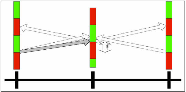
Figure 4. Offset Change Impacts.
In this example, the offset of the middle intersection is adjusted downward (earlier). Notice that this impacts the right-bound traffic flowing to the right intersection, as well as the two links of left-bound traffic.
There is always a temptation to adjust the offset at one intersection to accommodate demand in one direction on one link without taking into account the effects of this change on the other three links. One way to manually analyze the offset impacts is to use the Kell Method described below.
One-Way Offset
For the predominant one-way flow situation, the expedient approach requires only an estimate of the median travel time between intersections. The offset, expressed in seconds, is set at the intersections farthest upstream to an arbitrary value—many engineers use 0 seconds. The offset at the nearest downstream intersection is determined by adding the travel time to the offset of the adjacent upstream intersection. The travel time is estimated by dividing distance between the intersections by the average speed on the link. This process continues until the offsets of all intersections in the group have been determined.
Notice that this method of determining offsets is independent of the splits at each intersection and the cycle length.
As a further refinement, many traffic engineers will provide sufficient time for any standing queue to discharge before the arriving platoon. To do this, estimate the total number of vehicles in queue (vehicles that arrive during the red and do not turn right). Divide this number by the number of lanes, and multiply the result by 2.5 seconds. Subtract this total from the offset that was determined by the link travel time. Adjusting for the average standing queue is referred to as the “Smooth Flow Offset.” As with the basic offset calculation method, when adjusting for the standing queues, start at the upstream intersection and work downstream calculating each offset based on the upstream offset by adding the travel time and subtracting the queue discharge time to the upstream offset at each intersection.
Two-way Offsets (Kell Method)
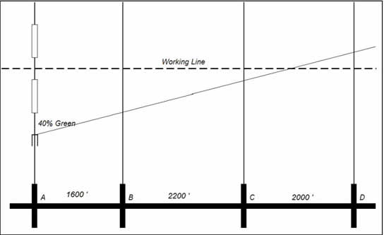
The Kell Method is a technique that can be used to manually construct a Time-Space Diagram that results in balanced offsets in both directions. This technique is named after its developer; Mr. James H. Kell, who was an instructor at University of California, Berkeley. The process is straightforward and requires a minimum input of information. An estimate of the percent green for the main street for each intersection, the average speed on the arterial, and the distance between intersections are the only information required to use the technique. The products of the method are the cycle length for the arterial and the offset for each intersection that provides equal bandwidth in each direction. The process is as follows:
Prepare a scale drawing laying out the intersections along the bottom of the page.
Draw a vertical line at the first intersection on the left.
Draw several cycles on the vertical line using a closed rectangle to represent the percent of time that the signal is NOT green.
Draw a horizontal working line through the middle of either a green or not-green.
Draw a line that slopes upward and to the right at the beginning of green at the left-most intersection. The sketch would look something like that shown in Figure 5.
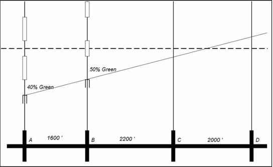
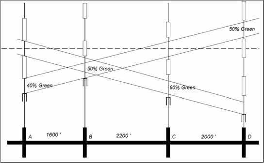
Figure 5. Kell Method (Beginning).Plot the cycle of the next intersection such that either the green or the not-green (whichever causes the beginning of green to come closest to the sloped line) is centered on the Working Line, as shown in Figure 6.
Figure 6. Kell Method (Continued).Continue plotting the cycle for the remaining intersections by centering either the green or the red. A completed diagram is shown in Figure 7.
Figure 7. Kell Method (Completed Diagram).Notice that this technique forces a symmetrical solution that provides two-way progression with approximately equal bandwidths in each direction. The final step in the process is to determine the cycle length. In general, traffic will move on an arterial at a speed that the drivers consider reasonable for the prevailing conditions. The Engineer must estimate this speed and use it to determine the cycle length. Notice that the diagram shows that a vehicle requires approximately 1 ½ cycles to travel from intersection “A” to “D” in either direction. If the prevailing speed on the arterial were 35 MPH, then an appropriate cycle length would be 75 seconds. This is determined by noting that it requires 1 ½ cycles to travel 5,800 feet which is equivalent to 3,867 feet per cycle. The cycle length is determined by dividing the distance (3,867 feet) by the speed, 51.33 feet per second (35 MPH), and the cycle is 75 seconds.
Split Issues
The split is the amount of time allocated to each phase in a cycle at each intersection. The toolbox offers two ways to calculate splits manually, the Greenshields-Poisson method previously described and the Critical Movement method which is described below.
Critical Movement Method
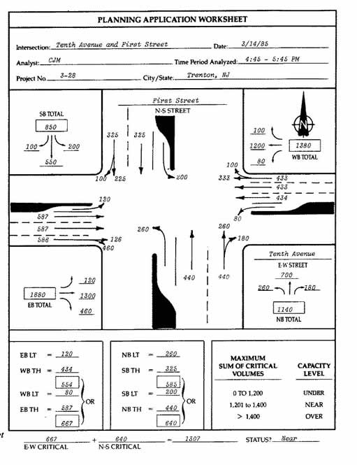
This method uses techniques that were employed in the 1984 Highway Capacity Manual as a “Planning Analysis” (Figure 8) to estimate intersection capacity. We have adapted elements of this analysis to use to develop traffic signal timing parameters. To use this method, intersection turning movements, the signal phasing, and the cycle length for the intersection must be known. The designer must determine the effective demand for each phase by applying various adjustment factors to reduce the demand to passenger car equivalents per lane.
For the purposes of preparing traffic signal timing plans, a high level of precision is not needed. Traffic demand can vary plus or minus 20 percent in just a few minutes at a given location. Also a variation of 20 percent from day to day is not unusual. Our objective, therefore, is to develop timing plans that are robust and that will perform well through a wide range of demand conditions. The following steps are suggested:
If the left turn movement is not protected, multiply the left turn demand by 1.6.
If the number of trucks is known, multiply the trucks by 1.5.
Divide the traffic demand on the four major and left-turn approaches by the number of lanes for each movement.
Determine the critical movements for both the east-west street and the north-south street. Determine the intersection critical movement by adding these two together. If this sum is less than 1,500, then continue. If it is over 1,500 then the intersection is probably over-saturated and the method may not be applicable.
Determine the number of critical movements in each cycle. With no left-turn protection, there would be two; with left turn protection on one street there would be three; and with left turn protection on both streets there would be four. Multiply the number of critical movements by five (the lost time), and subtract this number from the cycle length. This result is an estimate of the total available seconds of green per cycle that can be used for traffic movements.
Figure 8. Critical Lane Analysis Example.The final step is to multiply the total available green time by the ratio of the critical lane volume for the movement to the total intersection critical lane volume. For pre-timed operation, this is the phase green time in seconds. For coordinated operation with actuated controllers, this phase time is used to set the Force-off for the phase. For all actuated phases, the calculated time is the average green time for the phase. The phase maximum should be set at 25- to 50-percent greater than this value.
3 Maher, M.J. “Estimating the Turning Flows at a Junction: A Comparison of Three Models,” Traffic Engineering and Control 25 (11), pages 19-22.
4 “Comparison of Alternative Methodologies to Determine Breakpoints in Signal Progression,” TRB Paper by David Hook and Allen Albers, 2002.
5 The critical phases are the ones that require the most green time. The flow ratio is calculated by dividing the volume by the saturation flow rate for that movement.
6 The critical lane or movement for each phase is the lane that requires the most green time.
7 “Resonant Cycles in Traffic Signal Control;” Shelby, S.G., Darcy Bullock, and Douglas Gettman, TRB Meeting, January 2005.