
U.S. Department of Transportation
Federal Highway Administration
I. Introduction
Research and experience has shown that retiming traffic signals is one of the most cost-effective tasks that an agency can do to improve traffic flow. Traffic flow improvements of up to 26 percent have been reported.1 In spite of this potential, many Traffic Engineers simply do not have the budgetary resources to conduct a signal retiming program using the conventional methods.
The conventional approach to signal timing optimization and field deployment requires current traffic flow data, experience with optimization models, familiarity with the signal controller hardware, and knowledge of field operations including signal timing fine-tuning. To many practitioners, this is a daunting process that is best left to be performed by others at a time in the indefinite future. Setting new signal timing parameters for efficient traffic flow is time consuming and expensive. Typically, this process involves five distinct steps:
- Organizing existing information,
- Collecting new traffic flow data in the field,
- Coding and running signal timing optimization program(s),
- Validating and selecting optimum signal timing settings, and
- Installing and fine-tuning new signal timing plans in signal controllers in the street.
There are, however, practitioners in the field who have developed practical and cost-effective means to shortcut these tasks, and still generate signal timing plans that can approximate the effectiveness of signal timing developed using the formal modeling process. We refer to these plans as “near-optimum” plans. It is not reasonable to expect the same quality signal timing output from a shortcut method as from the formal, costly process. However, when faced with a lack of resources such that signal timing by conventional means is not possible, these shortcut methods should be considered—rather than not retiming the signals.
This report examines the informal traffic signal timing process and defines the various methods that can be used to minimize the cost of generating near-optimum signal timing settings. This effort places a primary emphasis on updating the signal timing in an arterial corridor. In short, this effort investigates how signal timing plans can be developed and updated efficiently at the lowest possible cost.
Intended Audience
The intended audience for this report includes administrators, managers, engineers, and technicians who are trying to maintain the best possible signal settings with less than optimal budgets. The report assembles a body of knowledge related to signal timing that is structured to be useful to those who are responsible for making the constant signal timing adjustments that necessary to meet the ever-increasing traffic demands.
Classical Signal Timing Process
Signal timing is a task that frequently involves coordinating activities of many different departments of the jurisdiction. For example, it is not unusual for the Planning Department to provide the traffic counts and mapping data, and for the Traffic Engineering Department to conduct the timing optimization analysis, with the Maintenance Shop performing the actual parameter installation. It is important to recognize that the signal timing process is not simply executing a computer program; rather, it is a continuing series of tasks that involve persons with many different skills. Two of the most prominent are the traffic engineer and the traffic signal technician. The engineer typically uses a software model, such as PASSER™ II or Synchro, to derive the timing plan, which is defined in terms of a cycle length, split, and offset. These data are then provided to the traffic signal technician who must convert these variables into the timing parameters used by the controller.
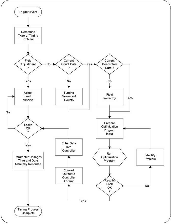
It is useful to examine the entire signal timing process as it is commonly practiced today in many cities and counties. The complete process is probably more complex than one might expect. Figure 1 illustrates the major activities and interfaces that are typically followed to update signal settings. Whether the process is applied to a single intersection or to an entire city, the steps are the same. It is also interesting to note that the same steps must be followed whether the process is entirely manual or completely automated. Each of the major activities of the signal timing process is described below.
In the real world, the signal timing process begins with a “Trigger Event.” This event may be as benign as a scheduled activity to retime the controller every few years. More likely, however, the impetus for new signal timing is a citizen complaint (e.g., “The light is too short”); a major change in the road network (e.g., widening of the existing arterial); or a significant change in demand (e.g., opening of a shopping center). Whatever the cause, the initial response is usually a review of the existing timing and equipment to ensure there is no hardware failure. One of the most common signal timing complaints is that the phase time is too short. This is frequently a result of a detector malfunction. The initial response, then, is to confirm that the hardware is operational and the timing parameters are operating as planned. After the Trigger Event, there are two basic paths through the process: Field Adjustments and System Retiming.
The “Field Adjustment” path is shown in Figure 1 as the path directly below the “Determine Type of Timing Problem” box. This path is entirely empirical and intuitive and produces results only as good as the experience of the person performing the adjustments. The other path is the one on which we will focus most of our attention. This path begins with a data collection effort and continues through an optimization process to generate and install new system timing parameters. There are three primary activities involved in the Classical Signal Timing Process: Data Collection, Optimization, and Installation/Evaluation.
Data Collection
Signal retiming is not making simple adjustments to a few timing parameters in a controller. Most jurisdictions follow a more complicated effort to retime a signal or group of signals using modern computer programs and procedures. This path involves the more complex activities that are indicated in Figure 1 to the right of the “Field Adjustment” path. There are two broad categories of data that are required by the process: turning movement counts and network descriptive data. The user must maintain accurate records of all timing input data for this process to be effective.
Figure 1. Classical Approach to Signal Timing.
Turning Movement Counts
This path through the flow chart begins with a determination of whether there is adequate traffic count data. For the most part, the necessary data includes turning movement counts that reflect the traffic demand. Most traffic engineers consider four plans to be the minimum required for proper signal operation: AM peak plan, day plan, PM peak plan, and night plan. Therefore, a basic needis to have a turning movement count for each of these four periods. In areas near major shopping venues there may be additional needs for unique timing plans that are related to shopping demand.
While this seems simple enough, it is not inexpensive. Collecting these data typically costs in the range of $500 to $1,000 or more per intersection. Converting the raw count data into a format useful for analysis easily can double the cost. This is an area where significant progress has been made. For example one vendor, Jamar Technologies Inc., makes an electronic data collection board that is easy to use, accurate, and reliable. Although an observer is still required to record the movements, once the observations are completed, the data are easily uploaded to a computer for further processing.
The more elegant solution to this problem, however, is to collect the data using existing system and local detectors and derive a complete traffic volume network with all turning movement from these detector data. Several systems, such as QuicNet/4, MIST, Pyramids, and Actra (and there are likely others), have the capability to export traffic count data from existing count stations. The missing capability is to be able to use this information to build a complete network turning movement schedule.
Traffic count data must be considered in two dimensions: temporal and spatial. In the temporal dimension, traffic count data at any one point varies from period to period as traffic demand ebbs and flows. In the spatial dimension, we frequently require traffic count data at many different intersections for the same time period. In addition, to accommodate certain flows through a series of intersections, we need to know the upstream origin of the demand for each turning movement at the downstream intersection.
The need for traffic counts is not a unique demand for signal timing; most Traffic engineering endeavors require traffic count information. Traffic signal timing, however, does require accurate turning movement counts.
Turning movement counts (or estimates) are fundamental to developing timing plans. These counts must be estimated in such a way as to represent traffic demand. In other words, one must be sure that the count information truly represents traffic demand and not just the traffic that was able to get through the intersection with the existing signal settings. A related issue to be aware of is the possibility that the traffic counted on a particular approach is actually constrained by the signal settings at the upstream intersection feeding that approach.
Descriptive Data
All signal optimization and simulation models, even manual signal timing procedures, require a physical description of the network. This description includes distance between intersections (link length), the number of lanes, lane width and grade, permitted traffic movements from each lane, and the traffic signal phase that services the flow. Building a network from scratch is a significant undertaking. But once the network is defined, in general, only traffic demand and signal timing parameters have to be updated to test a new scenario.
An implied issue in this step is identification of which intersections are to be included in the system. While this is a trivial issue for many simple networks, it can be a difficult problem to resolve in the more complex networks. In general, signals should operate as a system when adjacent intersections have similar cycle length requirements and there are significant benefits to be derived from controlling the offset. When the cycle length requirements are within 15 seconds of one another and the distance between intersections is less than 0.5 miles, many traffic engineers feel that the signals should be coordinated. These issues will be explained in more detail in later sections of this document.
Optimization
Once the data are collected, the final step is to generate the optimized signal settings. While this task can be accomplished manually (later sections of this report describe some manual techniques), most engineers use a computer program. There are a number of computer programs that can be used to generate signal timing parameters. These programs can be placed into one of two categories: those developed by the private sector and those developed by the public sector. The programs developed by the private sector tend to be more expensive to purchase but also tend to be updated more frequently. The programs developed by the public sector tend to be more thoroughly vetted by the research community. Three of the more popular programs of this type are Synchro, PASSER™ II, and Transyt-7F. The Federal Highway Administration's (FHWA's) Traffic Analysis Toolbox provides additional resources (http://www.ops.fhwa.dot.gov/trafficanalysistools/toolbox.htm).
Synchro
Synchro is a macroscopic traffic signal timing tool that can be used to optimize signal timing parameters for isolated intersections, arteries, and networks. It produces useful time-space diagrams for interactive fine-tuning. Synchro can analyze fully actuated coordinated signal systems by mimicking the operation of a National Electrical Manufacturers Association (NEMA) controller, including permissive periods and force-off points. Using a mouse, the user can draw either individual intersections or a network of intersecting arteries, and also can import .DXF map files of individual intersections or city maps. The program has no limitations on the number of links and nodes.
Synchro is designed to optimize cycle lengths, splits, offsets, and left-turn phase sequence using proprietary logic. The program also optimizes multiple cycle lengths and performs coordination analysis. When performing coordination analysis, Synchro determines which intersections should be coordinated and those that should run free. The decision process is based on an analysis of each pair of adjacent intersections to determine the “coordinatability factor” for the links between them.
Synchro calculates intersection and approach delays either based on the Highway Capacity Manual (HCM) or a proprietary method. The major difference between the HCM method and the Synchro method is treatment of actuated controllers. The HCM procedures for calculating delays and level of service (LOS) are embedded in Synchro; thus, the user does not need to use HCM software.
Synchro has unique visual displays, including an interactive traffic flow diagram. The user can change the offsets and splits with a mouse, then observe the impacts on delay, stops, and LOS for the individual intersections, as well as the entire network.
PASSER™ II
PASSER™ II (Progression Analysis and Signal System Evaluation Routine) was originally developed in 1974 by the Texas Transportation Institute (TTI). PASSER™ II is an arterial-based, bandwidth optimizer, which determines phase sequences, cycle length, and offsets for a maximum of 20 intersections in a single run. Splits are determined using an analytical (Webster’s) method, but are fine-tuned to improve progression. PASSER™ II assumes equivalent pre-timed control.
PASSER™ II requires traffic flow and geometric data, such as design hour turning volumes, saturation flow rates, minimum phase lengths, distances between intersections, cruise speeds, and allowable phase sequencing at each intersection. The PASSER™ II timing outputs include: design phase sequences, cycle length, splits, and offsets, and include a time-space diagram. Performance measures include volume-to-capacity ratio, average delay, total delay, fuel consumption, number of stops, queue length, bandwidth efficiency, and LOS. In addition to the time-space diagram, PASSER™ II has a dynamic progression simulator, that allows the user to visualize the movement of vehicles along the artery using the design timing plan.
There are two other versions of PASSER™ that are available, PASSER™ III and PASSER™ IV. PASSER™ III is a diamond interchange signal optimization program and PASSER™ IV is a program that is used to optimize a network of traffic signals that is based on maximing bandwidths.
Transyt-7F
Transyt-7F (TRAffic Network StudY Tool, version 7, Federal) is designed to optimize traffic signal systems for arteries and networks. The program accepts user inputs on signal timing and phase sequences, geometric conditions, operational parameters, and traffic volumes. Transyt-7F is applied at the arterial or network level, where a consistent set of traffic conditions is apparent and the traffic signal system hardware can be integrated and coordinated with respect to a fixed cycle length and coordinated offsets. Although Transyt-7F can emulate actuated controllers, its application is limited in this area.
Transyt-7F optimizes signal timing by performing a macroscopic simulation of traffic flow within small time increments while signal timing parameters are varied. Design includes cycle length, offsets, and splits based on optimizing such objective functions as increasing progression opportunities; reducing delay, stops, and fuel consumption; reducing total operating cost; or a combination of these.
Unique features of Transyt-7F include the program’s ability to analyze double cycling, multiple greens, overlaps, right-turn-on-red, non-signalized intersections, bus and carpool lanes, “bottlenecks,” shared lanes, mid-block entry flows, protected and/or permitted left turns, user-specified bandwidth constraints, and desired degree of saturation for movements with actuated control. Other applications of the tool include evaluation and simulation of “grouped intersections” (such as diamond intersections and closely-spaced intersections operating from one controller) and sign-controlled intersections.
Of course, this power and flexibility comes with a price. This is by far the most complex program to set up and use. It is also the most expensive and probably not the best selection for developing signal timing plans with a minimum budget.
Installation and Evaluation (Field Adjustments)
Once the hardware is determined to be operating correctly, the last task is to evaluate how well the new signal settings are managing traffic demand. Often, a simple adjustment of one parameter is all that is necessary. It may be possible to accommodate longer queues on the main street, for example, by simply advancing the Offset by several seconds. Other timing problems can be resolved by simple adjustments to the Minimum Green or Vehicle Extension parameters. These types of issues are resolved by a positive output from the “Field Adjustment” decision in Figure 1. In most jurisdictions, the entire sequence, from determining the type of problem, to making the adjustments, to evaluating the results, and to recording the changes is a manual process that relies on the experience of a signal engineer (or signal technician) to provide a solution. Obviously, the quality of the solution is a function of the experience and dedication of the person performing the work.
Report Structure
In addition to this introductory section, the report has five sections. Section II defines the eight steps that are common to any signal retiming effort, whether it is for one signal or for a system of hundreds of signals. When reviewing these steps, it is important to recognize that they exist whether or not they require any resources with the current effort.
This report provides a number of “rules of thumb” and methods that may be used to estimate various values that are used in the signal timing process. We caution the user to follow suggestions when appropriate, but to be aware that it is always desirable to verify these estimates with field observations when possible.
Section III provides a “tool box” of resources for the Practitioner. These resources will aid the user in collecting and managing data, and in better understanding the physical constraints involved with signal timing, and will explain back-of-the-envelope techniques that may be used when cost constraints prohibit more traditional solutions.
Signal settings can be categorized as local controller parameters or coordination parameters. The local controller parameters include phase minimums, extension times, and change and clearance intervals. Coordination parameters are the cycle length, split and offset. Section IV presents the local controller parameters and Section V discusses the coordination issues. Finally, Section VI provides three examples of how these techniques can be applied. One scenario involves an agency that has funds for signal timing but does not have enough resources to complete the classical method. The second scenario illustrates how an agency can develop signal settings with a modest budget, and the third scenario illustrates what an agency can do with virtually no budget for signal timing other than the part-time effort from existing staff.