Application of Travel Time Data and Statistics to Travel Time Reliability Analyses: Handbook and Support Materials
Chapter 2. Data Sources for Reliability
This section documents the data sources and collection methods for producing travel time values. These values are the basis for developing the travel time distribution from which reliability measures are derived. The discussion in this section focuses mainly on emerging data sources, especially the trajectory data now available from travel time vendors. The state of the practice is limited in many respects primarily because, up to only recently, most of the continuously collected data that have been available do not represent true travel times as measured by vehicle movement.
Freeway Detectors
Freeway detectors have been a source of speed data for several decades:
- Sensor: A variety of collection methods exist, including inductive loops, microwave radar, active infrared, passive infrared, acoustic array, and video image processing.
- Spatial attribute: Point
- Temporal attribute: Continuous
- Measurement type: Instantaneous—measurements are aggregated in the field at 20-second intervals.
- Direct data measurements: All of the sensors can produce volume, lane occupancy on a lane-by-lane basis at specific points. Inductive loop, microwave radar, active infrared, and video image-processing sensors also can provide vehicle classification, though some sensor types (e.g., radar) only provide length-based classifications rather than the Federal Highway Administration (FHWA) Traffic Monitoring Guide’s 13-class scheme.4
- Indirect measurements derived from data: Speed, travel time
- QC methods: Sensor outages or other events could result in missing or erroneous data at various dates and times. Active infrared, passive infrared, and video image-processing performance is affected by inclement weather, such as heavy rain, snow, and dense fog. Likewise, depending on placement and configuration, low-speed traffic movement can influence radar measurements.
The American Association of State Highway and Transportation Officials (AASHTO) Guidelines for Traffic Data Programs recommends that the QC process includes one or more of the following actions:5
- Reviewing the traffic data format and basic internal consistency
- Comparing traffic data values to specified validation criteria
- Marking or flagging traffic data values that do not meet the validation criteria
- Reviewing marked or flagged traffic data values for final resolution
- Imputed marked, flagged, or missing traffic data values with best estimates (while still retaining original data values and labeling imputed values as estimates)
Common validation criteria for freeway detector data include the following:
- Univariate and multivariate range checks—Involves validating data against an expected minimum, maximum, or range of expected values for a single variable (e.g., volume, occupancy, or speed) or a combination of variables (e.g., maximum consecutive identical volume, occupancy, and speed values, combinatory checks).
- Spatial and temporal consistency—Involves validating the consistency of data compared to adjacent locations (either across lanes or upstream and downstream monitoring locations) or previous periods.
- Detailed diagnostics—Involves validating individual vehicle data at a detector location using detailed diagnostic tests, such as individual vehicle velocity versus moving median velocity and headway versus on-time feasible range of vehicle lengths. These criteria entail detailed diagnostic data from traffic detectors that are typically not available from archived data sources.
Turner recommended the following validity criteria for detector data (table 1) ) in the report titled, "Quality Control Procedures for Archived Operations Traffic Data: Synthesis of Practice and Recommendations."6 Turner also recommended the following practices:
- Recognize that validity criteria are only one part of a comprehensive quality assurance process that does more than just discard suspect data that already have been collected
- Provide metadata to document QC procedures and results
- Provide metadata to document historical traffic sensor status and configuration
- Use database flags or codes to indicate failed validity criteria
- Implement, at a minimum, a basic foundation for data validity criteria (table 1)
- Further develop other spatial and temporal consistency criteria for detector data
- Use, when feasible, visual review to supplement the automated validity criteria
- Processing procedures: Travel times between detectors are assumed based on spot speeds.
Table 1. Validity criteria for freeway detector data.7
Validity Criteria |
Default Parameters |
| Prescreening criteria |
– |
| Controller error codes (e.g., −1, 255, etc.) |
N/A |
| Check consistency of elapsed time and poll cycles |
N/A |
| Check for duplicate records (location identification (ID), date, time identical) |
N/A |
| If volume = occupancy = speed = 0, then set speed = missing/null (no vehicles present) |
N/A |
| Univariate range criteria |
– |
| Minimum volume |
Zero vehicles |
| Maximum volume |
3,000 vehicles per hour per lane (adjust for appropriate time interval) |
| Minimum occupancy |
0 percent |
| Maximum occupancy |
100 percent |
| Minimum speed |
0 miles per hour (mph) |
| Maximum speed |
100 mph |
| Multivariate logical consistency |
– |
| Maximum consecutive identical volume and occupancy and speed values (including volume = occupancy = speed = 0) |
Number of reporting intervals that corresponds to 30 consecutive minutes (maximum) with no vehicles detected |
| If volume > 0 and speed = 0 then invalid |
N/A |
| If volume = 0 and speed > 0 then invalid |
N/A |
| If volume = speed = 0 and occupancy > 0 then invalid |
N/A |
| If occupancy = 0 and volume > volumemax (based on maximum possible volume when occupancy value is truncate to 0) |
Volumemax = (2.932×SPEED×ELAPSED_TIME)/600 |
– = no data; N/A = not applicable; ID = identification.
The lane-by-lane detector volumes and spot speeds are translated into station-, link-, and facility-level statistics using the following steps:8
- Freeway detector data is aggregated in the field to 20- or 30-second averages (speeds and lane occupancies) and sums (volumes). These are usually further aggregated to 5-minute intervals.
- For each 5-minute interval, the lane-by-lane data at each detector location are combined into a station across all lanes in a direction. The traffic volume is summed across all lanes, while a weighted average speed is calculated based on traffic volume in each lane. The weighted average speeds represent the time-mean speeds at a specific station.
- The 5-minute station data are expanded to links by assuming that each detector has a zone of influence equal to half the distance to the detectors immediately upstream and downstream from it. The measured speeds and volumes are assumed to remain constant within each zone of influence, and travel times along each link are calculated by dividing the equivalent link length by the average travel speed.
- The 5-minute link data are aggregated with adjacent links to form analysis facilities. The beginning and end points of the analysis facilities are based on logical breakpoints, such as major highway interchanges or other locations where traffic conditions are expected to change because of traffic or roadway characteristics. Facility travel times for each 5-minute interval are calculated as the summary of link travel times. Whenever a link travel time is missing, the whole facility travel time for that 5-minute interval may be set to a null value. To minimize the harmonic fluctuations associated with speed data, an average facility speed for each 5-minute interval is calculated as the facility length divided by facility travel time. These speeds represent space-mean speeds across the analysis facility.
Traffic Signal Detectors
- Sensor: Advanced controllers in signal cabinets record high-resolution signal event data that consist of a log of discrete events such as changes in detector and signal phase states.
- Spatial attribute: Point
- Temporal attribute: Every 0.1 second
- Measurement type: Signal event data are recorded at the highest time resolution of the controller (0.1 second). The signal controller-generated events are outputted in sets of four bytes per event: one byte for the event code type, one byte for the event parameter (for signifying detector numbers and phases), and two bytes for the timestamp of when the event occurred. The event code type specifies the type of event that occurred:
- Event code IDs 0–20. Active phase events: Indicate phase-related status changes, such as activation or termination
- Event code IDs 21–30. Active pedestrian phase events: Indicate pedestrian-related phase status changes
- Event code IDs 31–40. Barrier/ring events: Indicate barrier and yellow permissive events
- Event code IDs 41–60. Phase control events: Indicate phase hold, call, and omit status changes
- Event code IDs 61–80. Phase overlap events: Indicate overlap status changes
- Event code IDs 81–100. Detector events: Indicate detector activity and error status changes
- Event code IDs 101–130. Preemption events: Indicate preemption status changes
- Event code IDs 131–170. Coordination events: Indicate coordinated timing status changes, such as cycle length and split times
- Event code IDs 171–199. Cabinet/system events: Indicate controller property-related status changes, such as alarms, clock updates, and power failures
- Event code IDs 200–255: User-defined events: Indicate user-defined events
- Direct data type measurements: Data types include signal event data, cycle times, and phase intervals.
- Indirect measurements derived from data: Direct data can be integrated with vehicle count event data to produce measurements for delay, queue length, and green/red occupancy ratio.
- QC methods: They include hardware maintenance that enable proper collection of high-quality event data and communications systems that ensure signal controller clocks are synchronized. The QC process also includes ensuring proper coordination of inductive loop detectors to the signal detectors.
- Processing/calculation procedures: Day, et al. documented a workflow for developing operational performance measures from postprocessed signal event data, as shown in figure 2.9 The first step is to obtain event data from the field. The next step is to extract the cycle times and phase intervals from the data, which provides the set of relevant time intervals to support performance measurement. Once the cycles and phase intervals are defined, it is possible to integrate the vehicle count event data to yield measures of effectiveness (MOE) as follows:
- Produce visualizations: The raw event data yields several graphical tools for characterizing signal performance, such as flow profiles and coordination diagrams.
- Compute vehicle MOEs: Vehicle counts are compiled on any phase with a working count detector. These support cycle-by-cycle performance measures for a lane, lane group, or phase.
- Compute estimated delay: A record of vehicle arrivals at the intersection can be measured using upstream or setback/advance detectors. This measure provides a means of estimating delay and queue length.
- Compute nonvehicle MOEs: MOEs for nonvehicle modes, such as pedestrians and transit vehicles, may be generated using Global Positioning System (GPS) trajectories of transit vehicles or pedestrian pushbutton actuation times.
The next step is to compile the cycle-by-cycle performance measures, which produces a series of data tables that may be aggregated for reporting purposes.
The report Performance Measures for Traffic Signal Systems: An Outcome-Oriented Approach documents the requisite data elements recommended for various performance measures.10
- Limitations: This method uses high-resolution data loggers at the signals and is thus available for a small percentage of signals that have this capability. It also is a very indirect method for deriving travel times. Unless it is integrated with re-ID detectors, it only gives delay at the signal and ignores segment travel times between intersections.
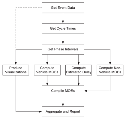
Source: Purdue University.
Figure 2. Flow chart. Performance measure analysis workflow.11
The steps (workflow) needed to convert detailed data collected by traffic signal controllers into performance measures: 1) Get Event Data; 2) Get Cycle Times; 3) Get Phase Intervals; 4a) Produce Visualization; 4b) Compute Vehicle MOEs; 4c) Compute Estimated Delay; 4d) Compute Non-Vehicle MOEs; 5) Compile MOEs; and 6) Aggregate and Report. Measures are computed for each phase interval in operation at the signal.
Vehicle Re-Identification Technologies: Bluetooth®, Electronic License Plate Readers, and Toll Tag Readers
- Sensor: There are a variety of collection methods, including Bluetooth® detection, electronic license plate readers (ELPR), and toll tag readers.
- Bluetooth® and wireless fidelity (Wi-Fi) detection systems use roadside readers to actively search for in-range devices and capture the unique Media Access Control (MAC) address of each device.
- ELPRs use optical cameras to capture images of license plates of oncoming or receding traffic and use video image processing to “read” the license plates. License plate numbers can then be matched at sensor locations downstream to generate travel times.
- Toll tag readers detect the unique radio frequency IDs of motorists’ automated toll tags at reader locations and calculate travel times based on the arrival time at each location.
- Spatial attribute: Line segment comprised reader pairs
- Temporal attribute: Continuous, but typically aggregated at 5-, 15-, 30-, and 60-minute epochs
- Measurement type: Travel times are directly measured based on a unique vehicle identifier (e.g., MAC address, license plate, or toll tag ID) and timestamp at fixed reader locations.
- Direct data measurements: All of the collection methods can produce vehicle travel times and speeds between reader locations.
- Indirect measurements derived from data: Travel time reliability and other travel time-based performance measures.
- QC methods: Variety of statistical methods developed primarily for ELPRs. Vendors typically have various methods of ensuring reasonable data, including removing errors and mixing in historical values to have smoother and fuller trendlines. However, most vendors consider these methods proprietary.
- Processing procedures: The travel time of an individual vehicle along a road segment is obtained by comparing the time when the vehicle is detected at the beginning of the segment to the time when the vehicle is detected at the end of the segment.
- Limitations: These data systems are based on the use of algorithms capable of discarding erroneous data. Data processing should account for unusual travel times caused by route choices, such as:
- Vehicle exits the facility to make an intermediate stop, then re-enters the facility later.
- Vehicle chooses an indirect route.
- Vehicle is detected at one device, undetected at next device, then detected at a later time or in the opposite direction.
- Penetration rate is relatively low (between 2 and 6 percent of traffic). Depending on local conditions, this method may not provide a statistically reliable sample of overall traffic speeds.
- Bluetooth® and Wi-Fi detectors do not provide lane-by-lane disaggregation.
Singer, et al. noted the following additional limitations:12
- Some Bluetooth® systems only report detected vehicles within a 10-second inquiry window, so all vehicles detected within this window will report the same detection time, leading to possible travel time inaccuracies, especially over short segment lengths. Each inquiry window could have up to eight detections, making it difficult for the system to match vehicles at multiple detector locations during heavy-traffic periods. However, newer generations of Bluetooth® detection systems utilize asynchronous input/output, allowing data to be output as soon as it is read.
- Accurate travel times depend on the spacing of readers. Long spacings can mask bottlenecks. For Bluetooth® systems, the nondirectional sensors may detect devices on nearby roadways, parking lots, and other surrounding areas. While data-processing algorithms can identify and remove much of the “noise” from the dataset, it is best to install readers such that unintended detections are minimized.
- ELPRs depend on a clear view of license plates; therefore, the system is sensitive to any factors that reduce visibility, such as precipitation, lens fog, line-of-sight obstructions, low ambient lighting, and license plates that are dirty, obstructed, missing, or have low character contrast. Not all State require vehicles to have a front license plate, so detection rates may be higher if rear plates are used.
- Toll tag readers are only feasible on routes where a significant percent of vehicles have toll tags. As with Bluetooth®, the appropriate positioning of toll tag readers is essential to achieve high detection rates. For example, multiple readers may be needed to cover all lanes of a roadway. However, a single reader may be sufficient if there is a large number of detectable vehicles and match rates are high enough to generate accurate travel times.
- Another consideration for toll tag readers is the potential for reader failure. Although device failure depends on many implementation factors (e.g., operating temperature, power conditioning), the potential for failure should be considered.
Vehicle Probe Data from Commercial Sources
- Sensor: Vehicle probe data is collected through a combination of GPS-derived vehicle locations and times, instantaneous speeds from onboard devices, and public agency detectors. These data are used to generate travel time information by aggregating the high-resolution raw data on vehicle locations in time and space. Several commercial vendors provide vehicle probe data. The National Performance Management Research Data Set (NPMRDS) is one such data set that FHWA makes available for use by certain public agencies.
- Spatial attribute: Polyline
- Temporal attribute: Various aggregations—Most typical ones being 5-, 15-, 30-, and 60-minute epochs (i.e., periods)
- Measurement type: Average travel time on segments aggregated by epoch. The segments are designated as traffic message channels (TMC) and roughly correspond to roadway segments between interchanges or intersections. Some vendors provide smaller geographic units than TMCs.
- Direct data measurements: None. Data are aggregated from direct measurements of GPS-equipped devices.
- QC methods: Appendix C of the National Cooperative Highway Research Program (NCHRP) Report 854 provides an example analysis of coverage, completeness, and validity for NPMRDS data.13 The coverage analysis compared the directional miles between the National Highway System NPMRDS geographic information system (GIS) map network and the full TMC-encoded network used by commercial sources. The completeness analysis examined the percentage of time data that was available for specific 5-minute periods. Finally, the validity analysis examined the differences between car and truck speeds. The researchers recommended to remove (or cap) speeds that were unreasonably high. An appropriate speed cap, if desired, should consider the functional classification of the roadway (freeway or arterial) and the speed data being investigated (“truck” or “passenger car” or “all vehicles”). After completing the QC process for the data, average speeds should be computed for the temporal and spatial aggregation levels desired:
- Establish free-flow (i.e., low volume) travel speed.
- Calculate congestion performance measures.
- Limitations: The current generation of vehicle probe data from commercial sources (e.g., NPMRDS version one and version two) are essentially spot speeds assigned to a link, and travel times are synthesized from these data. Travel times on a road segment are the average of vehicles; they do not reflect directly measured travel times except where path processing is used. This data source is not truly reflective of travel times over time and space. In addition, the raw data are aggregated data and not true measurements. This aggregation reduces the variability in the data, which is problematic for reliability calculations.
Some providers also may offer incident information, predictive travel time algorithms, and fusion of data from other sources (e.g., roadway sensors). One challenge of using vendor-provided data may be combining third-party data with data collected directly by a State or local agency (e.g., roadway sensor data).
Also, probe speed data does not capture travel times for every epoch of every road segment. Therefore, users typically have two overall choices to obtain data. One option is data that reflect direct field measurement and would contain measurement gaps when no probes are detected. The other would fill in these measurement gaps with imputed data. Using either choice has shortcomings. If one uses direct field measurements only, the road segments and epochs that have measurements may be reflective of higher traffic with lower speeds and greater unreliability, thereby over-representing these conditions in an aggregate analysis. On the other hand, using gap-filled data may artificially smooth the data in a way that would dampen fluctuation in the reliability analyses.
Lastly, while the TMC is theoretically a standard, TMC definition varies depending upon the vendor providing the data, making data integration challenging. Similarly, the TMC network may not fit transportation agency applications as it may span multiple major intersections. Typically, a time-consuming conflation effort is developed to integrate probe speed data with a department of transportation’s network.
Vehicle trajectory data: Recently vendors have started to make available the high-resolution data on vehicle locations in time and space. From these data, vehicle trajectories can be derived that overcome many of the assumptions of the widely available facility-specific travel times. With trajectory data, it is possible to compute the actual travel times of vehicles between points, e.g., origins and destinations for an entire trip.
Ride-Hailing Companies
- Sensor: Ride-hailing companies are sometimes considered nonstandard sources but are still a valuable (and underutilized) source of travel time data that State and local agencies could use. Zone-to-zone travel times are synthesized from GPS trace pings from drivers operating on a company’s network. All drivers use a smartphone to handle the logistics of their trips through a ride-hailing company’s network. In 2017, a ride-hailing company made its travel time data available to the public via its movement data analysis tool.14 All data is anonymized and aggregated to ensure no personally identifiable information or user behavior can be found using the tool.
- Spatial attribute: Polyline
- Temporal attribute: Continuous, but reporting is intermittent
- Measurement type: The ride-hailing company’s application records latitude, longitude, and a timestamp (date/time) every 4 seconds. These GPS trace pings are used to provide navigational routing, fare calculations, driver-rider matching, and user-experience elements (e.g., display the location of the ride-hailing company-affiliated vehicles in the ride-hailing company’s rider application). When aggregated, the GPS trace pings can be used to derive average travel times between zones in a given region.
- Direct data measurements: Data types include device/vehicle trajectories and paths. These data can be aggregated to produce average travel times between two zones for a given time and date. Zones defined for a region are commonly based on census tracts, traffic analysis zones, or neighborhoods.
- Indirect measurements derived from data: Travel time analyses and origin-destination matrices may be developed from these data.
- QC methods: Travel time statistics are removed for zone pairs that either do not meet:
- A minimum number of trips: In general, there should be at least five trips between origin and destination during the period examined.
- A minimum count of unique riders necessary to preserve rider privacy (e.g., at least three different customers)
- Limitations: Cortright noted several limitations to these data.15 The movement tool provides trip times only for origin-destination pairs that have a sufficient number of trips (undertaken by the ride-hailing company’s drivers) to enable them to calculate average trip times. While this is not a problem in dense, urban environments, data are sparse in lower density areas and for suburb-to-suburb trips. In addition, this ride-hailing company filters out trips that do not meet minimum thresholds for data privacy as well as origin-destination pairs that have fewer than 30 observations in a given month. Another limitation is that this ride-hailing company lacks data on traffic volumes.
Connected Vehicles
- Sensor: Vehicle-to-infrastructure communication allows vehicles and infrastructure to communicate with one another via dedicated short-range communications transceivers. Infrastructure can communicate location-specific or general messages to vehicles, such as curve speed warning, road condition warning, weather information, and incident/detour information. Vehicles can communicate their presence to infrastructure, enabling features such as traffic signal actuation, automatic toll payment, incident detection, and general information sharing (i.e., traffic volume and travel time).
- Spatial attribute: Varies
- Temporal attribute: Continuous
- Measurement type: A probe data breadcrumb log stores vehicle location, heading, speed, and path history as part of the basic safety message (BSM), as summarized in table 2. This information is stored on aftermarket safety devices (ASD) onboard the vehicle and is communicated to roadside units (RSU).
Table 2. Basic safety message core data fields.16
BSM Core Data Fields |
Description |
| msgCnt |
Message count |
| ID |
Temporary identification of vehicle |
| secMark |
Message time |
| Lat |
Latitude of vehicle |
| Long |
Longitude of vehicle |
| Elev |
Elevation of vehicle |
| Accuracy |
ASD estimation of location sensor accuracy |
| Transmission |
State of the vehicle’s transmission |
| Speed |
Vehicle speed |
| Heading |
Vehicle heading |
| Angle |
Steering wheel angle |
| accelSet |
Vehicle acceleration state in all three axes |
| Brakes |
Vehicle braking status |
| Size |
Vehicle size |
In addition, a finer path history called “crumbData” may be collected, as summarized in table 3.
Table 3. Crumb data fields.17
Optional CrumbData |
Description |
| elevationOffset |
The elevation offset from the BSM CoreData:elev field |
| Heading |
Vehicle heading at the time offset of this crumb |
| latOffset |
The latitude offset from the BSM’s CoreData:lat field |
| lonOffset |
The longitude offset from the BSM’s CoreData:lon field |
| posAccuracy |
Position accuracy with regard to multiple axes |
| Speed |
Vehicle speed at time = BSM time + this crumb’s time offset |
| timeOffset |
The time offset from the time of the parent BSM |
- Direct data measurements: The probe data breadcrumb data yields measurements of travel times at the vehicle level. The RSU travel time source data is collected from a single passing BSMs to facilitate travel time computations for the traffic control system. These data are limited and used by the transportation management center to develop link travel times to compare the connected-vehicle data with other travel time data sources.
- Indirect measurements derived from data: Not applicable
- QC methods: The Connected Vehicle Pilot Deployment Program Data Management Plans for Tampa, FL, and New York City, NY, outline key data quality attributes (i.e., validity, reliability, precision, integrity, and timeliness) to ensure data collected and produced in the pilot projects result in reliable analytical results.17,18 Scheduled and unscheduled data quality audits are conducted to identify erroneous data from data streams. Once discovered and assessed, there are three ways to process erroneous data:
- Delete—If it is determined that the data has no significant value or impact to the overall data set, application, or performance measure, the data may be deleted.
- Flag—If it cannot be determined that the data has significant value, cannot be parsed from its erroneous components, or impact to the overall data set, application, or performance measure is undetermined, the data may be retained but flagged to be omitted from certain analysis.
- Correct—If it is determined that the data have significant value, can be parsed from its erroneous components, or has a negligible impact on the overall data set, application, or performance measure, then the data may be retained. They can be flagged as corrected or further cleaned. Corrected data can be included or may be omitted from certain analysis.
Another critical component of data quality for the Tampa pilot is the configuration management plan, including procedures for submitting and approving any proposed design change. In addition, on ongoing log of current and historical configurations are documented, such as software and firmware versions/dates, device serial numbers, and maintenance and repair activities.
- Processing procedures: The BSM’s core data (and if configured, crumb information) is uploaded daily to the transportation management center through RSUs. Breadcrumb data structures are stored on the ASD and uniquely tagged and processed separately at the transportation management center for mobility analytics. Figure 3 depicts a high-level view of where and how data flows from ASDs and RSUs to the transportation management center for subsequent analysis, sanitization, analysis, backup, archive, and export.
- Limitations: These data provide the most direct measurement of travel times as experienced by users. This method relies on appropriate processing algorithms to achieve high accuracy. The data management plan for the pilots notes that the travel time data may be used at the transportation management center for measuring segment travel times where there is no instrumentation. A major limitation currently is the limited market penetration of this technology, leading to a lack of data for systematic analysis.
Summary of Travel Time Data Sources
Table 4 summarizes the characteristics of travel time data sources used for reliability analysis.
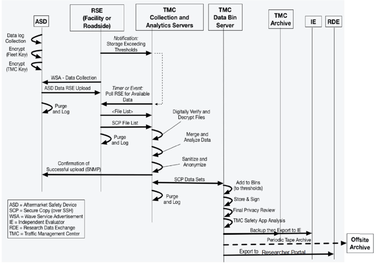
Figure 3. Diagram. Aftermarket safety device event and breadcrumb data collection and processing sequence.
Source: Federal Highway Administration, October 2017. Connected Vehicle Pilot Deployment Program Phase 2, Data Management Plan—New York City, FHWA-JPO-17-454.
Table 4. Characteristics of travel time data sources used for reliability analysis.
| Data Source |
Collection Method |
Measurement Type |
Data Types Derived from Measurements |
Quality Control Methods |
Processing Procedures for Reliability |
Limitations for Reliability Analysis |
| Freeway detectors |
Variety of detectors used: inductive loops, active infrared, passive infrared, acoustic array, and video image processing. |
Measurements are aggregated in the field at 20-second intervals. |
Volume, speed, lane occupancy on a lane-by-lane basis at specific points. Some methods provide vehicle classification. |
Univariate and multivariate range checks; spatial and temporal consistency; detailed diagnostics; checks against traffic flow equations. |
Travel times between detectors are assumed based on spot speeds. |
Point-based speeds are not truly reflective of travel times over time and space; aggregation reduces variability. |
| Traffic signal detectors |
Advanced controllers in signal cabinets record high-resolution signal event data. |
Signal event data (phasing, occupancy) are recorded at the highest time resolution of the controller. |
Signal event data, cycle times, and phase intervals. Data can be integrated with vehicle count event data to produce measurements for delay and queue length. |
None. |
Workflow includes getting event data, cycle times, phase intervals, produce measures of effectiveness (MOE), compile MOEs, and aggregate and report the results. |
Very indirect method of deriving travel times. |
| Bluetooth® detection |
Roadside readers actively search for in-range Bluetooth® devices and capture unique media access control addresses. |
Unique vehicle identifier and timestamp at fixed reader locations. |
Travel times and average speeds between reader locations. |
Variety of statistical methods developed primarily for ELPRs. |
Travel times between reader locations are directly measured. |
Depends upon algorithms capable of discarding erroneous data. Other limitations include inquiry window length, spacing of readers, sensitivity to environmental conditions, adequate saturation rates, and potential for reader failure. |
| ELPR |
Roadside readers optical cameras and video image processing to read license plates. |
Unique vehicle identifier and timestamp at fixed reader locations. |
Unique vehicle identifier and timestamp at fixed reader locations. |
Variety of statistical methods developed primarily for ELPRs. |
Travel times between reader locations are directly measured. |
Depends upon algorithms capable of discarding erroneous data. Other limitations include inquiry window length, spacing of readers, sensitivity to environmental conditions, adequate saturation rates, and potential for reader failure. |
| Toll tag readers |
Roadside readers detect the unique radio frequency identifications of motorists’ automated toll tags. |
Unique vehicle identifier and timestamp at fixed reader locations. |
Unique vehicle identifier and timestamp at fixed reader locations. |
Variety of statistical methods developed primarily for ELPRs. |
Travel times between reader locations are directly measured. |
Depends upon algorithms capable of discarding erroneous data. Other limitations include inquiry window length, spacing of readers, sensitivity to environmental conditions, adequate saturation rates, and potential for reader failure. |
| Vehicle probe data (epoch and segment based) from commercial sources |
Mix of: Global Positioning System (GPS)-derived vehicle locations and times; instantaneous speeds from onboard device; and agency detectors. |
Average travel time on segments aggregated to 1–5-minute intervals. |
Travel times by time interval (usually 1–5 minutes) and road segment. |
Range checks, analysis of coverage, completeness, and validity. |
Travel times on a road segment are the average of vehicles; They do not reflect directly measured travel times except where path processing is used. |
Segment-based travel times are not truly reflective of travel times over time and space; aggregation reduces variability. |
| Ride-hailing companies |
Zone-to-zone travel times are synthesized from GPS trace pings from drivers operating on the company’s network. |
The latitude, longitude, and a timestamp (date/time) are recorded every 4 seconds. |
Device/vehicle trajectories and paths. Average travel times between two “zones” in a region for a given time and date. |
Screening for minimum number of trips between zone pairs, or minimum count of unique riders. |
Zone assignment, mean epoch, zone to zone travel time, aggregate trips, privacy constraints, release. |
Trip times only available if sufficient number of trips are available within privacy constraints. Data are sparse in lower density areas and for suburb-to-suburb trips. Also lack of traffic volume data. |
| Connected vehicles |
Vehicle-to-infrastructure communication. |
Vehicle location and timestamp; these data are available today from telematics providers in over 4 million vehicles in the United States. |
Vehicle trajectories and paths. |
Key data quality attributes include validity, reliability, precision, integrity, and timeliness. Data quality audits are conducted to delete, flag, or correct erroneous data. |
Data flows from aftermarket safety device to roadside unit, and on to the transportation management center for subsequent analysis, sanitization, analysis, backup, archive, and export. |
Provide the most direct measurement of travel times as experienced by users. Rely on appropriate processing algorithms to achieve high accuracy. |
Travel Time Data Used in this Study
Common travel time data sources, including vehicle probe data, detector data and trajectory data, were investigated in this study. The NPMRDS (a private-firm version) was selected for the probe data, which includes field speed data for each TMC for timestamps at 5-minute intervals. Travel times on the TMCs are determined by tracking individual vehicles over a distance and then snapping these travel times to a TMC; this is known as “path processing.” Starting in 2017 (the period covered herein), the travel times in the NPMRDS are based on path processing. Both speeds and travel times are included in the data. Prior to 2017, the travel times were based on instantaneous or near-instantaneous vehicle speeds. The general data structure is shown in table 5.
Table 5. National Performance Management Research Data Set data sample, 2017.
|
Measurement_tstamp |
Speed |
| 106 + 05207 |
1/1/2017 0:25 |
63 |
| 106 + 05208 |
1/1/2017 0:25 |
64 |
| 106 + 05209 |
1/1/2017 0:25 |
64 |
| 106 + 05209 |
1/1/2017 0:30 |
62 |
| 106 + 05207 |
1/1/2017 0:35 |
65 |
| 106 + 05208 |
1/1/2017 0:35 |
64 |
Source: FHWA
Detector data capturing freeway traffic volumes and speeds was obtained from the California Department of Transportation’s (Caltrans) performance measurement system (PeMS) data. The data structure is similar to those of the probe data, except that data are collected on each detector station rather than TMC, as shown in table 6.
The Maryland State Highway Administration provided trajectory data from a private firm, which contain vehicle locations for short-interval timestamps of each recorded trip (as shown in table 7). Although speeds and travel times are not explicitly provided in the dataset, they can be calculated based on the location and time information.
Table 6. Detector data sample—California Department of Transportation performance measurement system, 2017.
Timestamp |
Station |
District |
Freeway |
Direction |
Lane_Type |
Length |
Total_Flow |
Percent_Observed |
Average_Speed |
| 1/1/2017 0:00 |
717075 |
7 |
10 |
E |
ML |
0.32 |
97 |
100 |
68.5 |
| 1/1/2017 0:00 |
717077 |
7 |
10 |
E |
ML |
0.235 |
108 |
100 |
69 |
| 1/1/2017 0:00 |
707097 |
7 |
10 |
E |
ML |
0.245 |
145 |
0 |
65.1 |
| 1/1/2017 0:05 |
717075 |
7 |
10 |
E |
ML |
0.32 |
83 |
100 |
68.1 |
| 1/1/2017 0:05 |
717077 |
7 |
10 |
E |
ML |
0.235 |
84 |
100 |
67.8 |
| 1/1/2017 0:05 |
717097 |
7 |
10 |
E |
ML |
0.245 |
118 |
0 |
64.6 |
Table 7. Trajectory data sample, 2018.
| Tripid |
Tstamp |
Latitude |
Longitude |
| 3f74eaa4-2e36-89be-dc6c-83530aa10bfe |
3/15/2018 3:51 |
38.990972 |
−77.157407 |
| eb8c3e25-4f3b-875a-44c0-a53e23911f66 |
3/14/2018 22:28 |
38.9906351 |
−77.1542528 |
| eb8c3e25-4f3b-875a-44c0-a53e23911f66 |
3/14/2018 22:28 |
38.9906902 |
−77.1545025 |
| eb8c3e25-4f3b-875a-44c0-a53e23911f66 |
3/14/2018 22:28 |
38.9908102 |
−77.1549984 |
| eb8c3e25-4f3b-875a-44c0-a53e23911f66 |
3/14/2018 22:28 |
38.9908704 |
−77.1552548 |
| eb8c3e25-4f3b-875a-44c0-a53e23911f66 |
3/14/2018 22:28 |
38.9909268 |
−77.155515 |
| eb8c3e25-4f3b-875a-44c0-a53e23911f66 |
3/14/2018 22:28 |
38.9909803 |
−77.1557819 |
| eb8c3e25-4f3b-875a-44c0-a53e23911f66 |
3/14/2018 22:28 |
38.9910564 |
−77.1563175 |
| eb8c3e25-4f3b-875a-44c0-a53e23911f66 |
3/14/2018 22:28 |
38.9910954 |
−77.1565785 |
|