Integrated Modeling for Road Condition Prediction Phase 3 Project Report

Chapter 3. Implementation and Deployment

Development of Integrated Modeling for Road Condition Prediction (IMRCP) capabilities presents diverse challenges. The interdisciplinary nature of the concept necessitates a broad group of stakeholders with particular operational needs, leading to an equally broad set of application scenarios. The variety of data types needed to support the scenarios requires identifying, accessing, and developing components for data collection from a wide variety of sources. The spectrum of data conditions, quality, and attributes across those sources then requires a flexible and extendable data repository and data processing capability to synthesize the input needed by all of the component forecast methods. The system and user interfaces should be able to represent the original data and forecast results in consistent, easy-to-use presentations that provide user-selectable geographical and past-present-future views.

As noted in the project description, previous phases of IMRCP have provided thorough analyses of the existing state of predictive methods in meteorology, traffic, hydrology, and operations planning. At the end of IMRCP phase 2, a prototype system integrating the data sources and methods needed to create predictions of system conditions was modeling part of the Kansas City metropolitan area and providing data to the Kansas City Scout transportation management center for evaluation. That deployment suggested certain enhanced capabilities that could improve the forecast results and user interfaces for operations and assessment. The resulting phase 3 deployment is described in this section.

User Needs

User needs for IMRCP were thoroughly described in the phase 1 analysis and concept of operations. Potential users of the IMRCP range from travelers to transportation operators to maintenance managers to consulting meteorologists to emergency planners. The breadth of interested stakeholders prefigures the wide range of functions to be required of the IMRCP.

Users need information to help them make appropriate travel and traffic management decisions. Too much information outside a user's context, however, may distract the user from more immediate and relevant information. Potential road condition predictions are useful only if they are relevant to the traveler's temporal and spatial context. This has significant ramifications for predictive capabilities. Traffic information provided to managers and travelers has, to this point, been limited to observed conditions, but predictions have more dramatic decision implications. Information must be timely enough to facilitate effective decisions based on anticipated conditions. Telling someone in the middle of a 1-hour (h) commute that severe congestion is likely for the next 30 minutes (min) is much less effective than having issued the advisory 90 min earlier.

Users need to have road condition predictions expressed in clear terms consistent with other similar contexts that help their decision-making processes. Traffic information and signage already provides some information of this type; travelers understand what an icy road ahead or a deer crossing sign means. These signs are used to express likelihood and provide an advisory appropriate to the traveler's immediate decision context. Predictive capabilities expand this concept to more specific times and conditions.

Application Scenarios

The potential users of IMRCP face diverse challenges related to traffic, weather, and hydrology. The IMRCP system functions can conceptually assist users in meeting these challenges.

Variable Speed Limits

Transportation systems management and operations (TSMO) practitioners could use IMRCP to be proactive rather than reactive. Dynamic or variable speed limits (VSL) can enhance network performance during peak demand periods when congestion and delay are often exacerbated by adverse weather, reduce traffic shock waves and incidents, and delay or prevent flow breakdown, and thus maintain optimal throughput. The posted speed limit, which could also consider visibility, friction, and traffic conditions, may be adjusted based on a combination of prevailing and predicted weather conditions.

Enhanced Traveler Information

Road weather information, such as in-route weather warning and route conditions, can be disseminated through radio, Internet, mobile devices, roadside dynamic message signs (DMS), and other similar means. Travel time predictions for alternative routes and times would enable users to select the best route and departure time for their particular travel need, including the impact of work zones or inclement weather. Travelers could therefore choose their departure time and/or route based on the predictive information.

Enhanced Intelligent Signal Controls

IMRCP integrates weather forecasts with traffic predictions. The results could form a basis for selecting traffic signal control interventions systematically. To achieve this, the signal control interventions would be linked to the predicted weather and traffic conditions based on measured conditions. Real-time traffic data feeds are used as a basis for the traffic state estimation and prediction within the IMRCP and could be obtained directly from signal control sensors in a corridor.

Maintenance

IMRCP enhances the ability to support strategic and tactical maintenance decisions at an agency. The IMRCP could complement the current use of MDSS at an agency by integrating traffic and roadway characteristics into a single predictive view of conditions. Using this integrated forecast enables agencies to make better decisions relating to winter maintenance. Similarly, IMRCP would provide non-winter maintenance personnel the capability to include weather and traffic forecasting in day-to-day decisions on maintenance scheduling.

Freight

IMRCP capabilities can help freight managers, dispatchers, and operators/contractors make better decisions in pursuit of higher customer satisfaction, at an overall lower cost. Once a truck is on the road for a long-haul move, whether for a truckload delivery or as part of a less-than-truckload (LTL) network move, predictive IMRCP information could help drivers select routes that best meet their travel time and travel time reliability objectives. Better route planning with IMRCP could then improve load planning by operators. This scenario, however, would require IMRCP to be deployed over an area consistent with the desired route planning.

Work Zones

For work zone personnel, IMRCP provides segment-level alerts for monitoring work zones. The tool complements the ability of smart work zones and work zone intelligent transportation systems (ITS) to provide more actionable information to travelers. Potential scenarios include near-term work zone support and coordination, where the work zone impact can be assessed using current conditions and imminent operations plans.

Travelers

As end-user beneficiaries of IMRCP, commuters will have access to forecasts of traffic conditions that parallel their access to weather forecasts. Commuters will also have access to predicted conditions resulting from planned (forecast) work zones, special events, or localized flooding.

IMRCP applications could enable tourists to plan long trips on unfamiliar roadway networks. Tourists would have access to traffic forecasting services in IMRCP that provide data for the entire trip planning horizon, predicting likely conditions using archived and real-time traffic conditions, and atmospheric and road weather forecast conditions. As in the freight scenario, this would require IMRCP to be deployed over an area consistent with the desired route planning.

Emergency Response

Just as IMRCP can facilitate predictive route planning for freight and individual travelers, it could also assist emergency response planning for either responders or evacuees. The model's predictions of traffic and roadway conditions, in consideration of weather and hydrology, could improve safety and mobility during incidents and, depending on severity, extreme weather events.

System Description

Because the purpose of IMRCP is to provide information on predicted road conditions, the user interface is essential to providing that view. IMRCP provides flexible reporting tools and an interactive map to meet that need. The data that populate these user interface features are kept in a data store that contains collected data and data generated through forecasting components. Forecast data are generated within the IMRCP context for traffic and road weather conditions and are obtained from sources outside the system for atmospheric weather, hydrology, work zone plans, and known special events. Current traffic and incident conditions come from the KC Scout advanced transportation management system (ATMS). Current environmental conditions are collected primarily from the National Weather Service (NWS) and other government agencies. The major system components and interfaces are illustrated in figure 1.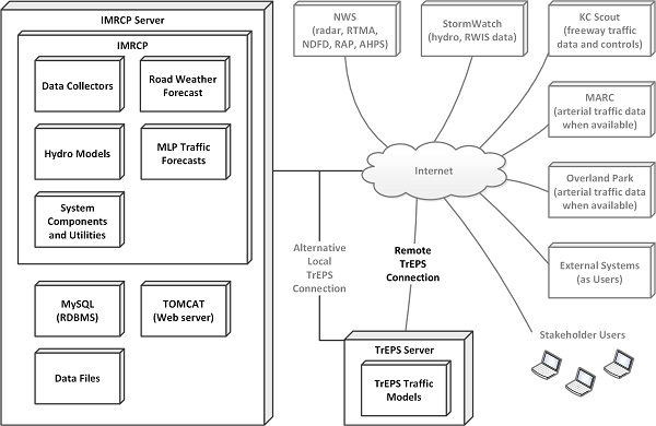

The figure depicts the IMRCP components and interfaces as configured for the Kansas City metro area demonstration deployment. Internet cloud branches out to NWS (radar, RTMA, NDFD, RAP, AHPS), StormWatch (hydro, RWIS data), KC Scout (freeway traffic data and controls), MARC (arterial traffic data when available), Overland Park (arterial traffic data when available), External Systems (as Users), Stakeholder Users, Remote TrEPS Connection, and IMRCP Server. Remote TrEPS Connection leads to TrEPS Server, including TrEPS Traffic Models, which also has an Alternative Local TrEPS Connection arm to the IMRCP Server. The IMRCP Server includes MySQL (RDBMS), TOMCAT (Web server), Data Files, and IMRCP. IMRCP includes Data Collectors, Road Weather Forecast, Hydro Models, MLP Traffic Forecasts, and System Components and Utilities.

AHPS = Advanced Hydrologic Prediction Service. IMRCP = Integrated Modeling for Road Condition Prediction. KC = Kansas City. MARC = Mid-America Regional Council.
MLP = machine learning-based prediction. NDFD = National Digital Forecast Database.
NWS = National Weather Service. RAP = Rapid Refresh. RDBMS = Relational Database Management System. RTMA = Real-Time Mesoscale Analysis. RWIS = road weather information system. TrEPS = Traffic Estimation and Prediction System.

Figure 1. Diagram. Components of the Integrated Modeling for Road Condition Prediction.
Source: Federal Highway Administration

Data Collection

The integration of diverse sets of data requires a diverse set of data collectors. Traffic, hydrology, and weather data relevant to a deployment area are collected from numerous sources.

Current air temperature, wind speed, surface pressure, and humidity observations are collected from the National Oceanic and Atmospheric Administration (NOAA) National Centers for Environmental Research (NCEP) Real-Time Mesoscale Analysis (RTMA). These weather observations are used as input to the traffic model for generating traffic predictions and to the road weather model for road weather predictions. They can be viewed on the map or through reports.

Atmospheric weather forecasts are collected from the NOAA NWS National Digital Forecast Database (NDFD). These forecasts are displayed on the user interface through the reporting and subscription features. They are also used in traffic and road weather predictions.

The NOAA/NCEP Rapid Refresh (RAP) is used as the source for forecast surface pressure, precipitation amount, and precipitation type. Forecast weather data are used for traffic and road weather predictions and providing information to users.

The NOAA National Severe Storms Laboratory (NSSL) Multiple Radar/Multiple Sensor System (MRMS) provides radar and precipitation rate and type observations for IMRCP. These weather data can be viewed on the map or through reports and are used as input for the traffic model and road weather prediction model.

Current hydrological conditions and forecasts are collected from the NOAA/NWS Advanced Hydrologic Prediction Service (AHPS) when new data become available at any of the AHPS stations in the study area. The values are used to determine the flood depth on road network links based on inundation mapping provided by AHPS. Additional hydrological conditions and forecasts for small streams can also be collected from other sources, when available.

The current pavement and subsurface temperatures can be collected from a road weather information system (RWIS) station or the Federal Highway Administration's Weather Data Environment (WxDE) for use in road weather predictions. These values are used in initiating road state and road temperature predictions with the Model of the Environment and Temperature of Roads (METRo).

Alerts, watches, and warnings are collected from NWS using the Common Alerting Protocol (CAP) and are available for IMRCP users to view.

Current traffic conditions are collected from traffic detectors maintained by the road network infrastructure owner/operator (in this case, KC Scout for the metro area highway network). Speed, volume, and occupancy data from these detectors are provided by an ATMS to the IMRCP system for predicting traffic across the network.

Incident and work zone data are also collected from an ATMS (again, KC Scout in this case). The location, estimated time frame, lane closures, and type of event are used to feed the traffic model for predictions and to display on the map.

Forecast Model Components

IMRCP forecasts traffic and road weather conditions using current and forecast atmospheric and hydrologic condition data from the data store, collected from the sources previously described.

The Traffic Estimation and Prediction System (TrEPS) model estimates and predicts the traffic demand and network states at the zone-to-zone (origin-destination) level. After an appropriate offline calibration based on traffic data archives for the network of interest, the TrEPS online component is capable of continuously interacting with multiple sources of current real-time traffic data, such as from loop detectors, roadside sensors, and vehicle probes, which it integrates with its own model-based representation of the network traffic state. TrEPS also considers and integrates current road weather conditions, incident status, and work zone plans into its estimation and prediction of network link speed, volume, occupancy, and travel times. For this IMRCP integration, detector, incident, work zone, and weather data input are provided from the core IMRCP data store.

The machine learning-based prediction (MLP) package predicts traffic network conditions given a set of system variables that include weather, work zones, incidents, and special events. MLP is a comprehensive, data-driven prediction module that uses a Markov process to explicitly characterize the probabilistic transition between traffic states under different external conditions (e.g., weather, incidents). For road network links without real-time traffic detectors, a neural network model is used for predictions if a detector can be matched within 5 miles downstream, and historical INRIX® data are used when no detector can be found downstream.

The METRo model estimates and predicts weather-related pavement conditions on roadways within the network of interest. The model computes pavement temperatures and surface conditions on network pavement segments and bridges using current condition data from RWIS and mobile sensors (when available), atmospheric weather forecasts, and pavement configuration data.

Data Store

All data collected and computed by the system are kept in its integrated data store. Data collected by the system directly from external sources are kept in their original formats. Data generated by the system in data digest and forecasting components are stored in compatible file structures. All data kept by the system are indexed to location and temporal contexts. All other system components work from data within the store for forecasting, presentation, and reporting. The data store was enhanced in phase 3 to provide faster access to large data sets in support of broader geographical views.

User Interface

The IMRCP user interface provides forecast traffic and road weather conditions on maps, on-demand reports, and in subscriptions. The map interface can be used to view conditions on roadways, over regions of a deployment area for alerts, in combinations. As a live system, the map can be set to view a single point in time or to automatically refresh as new data become available. Notifications of current events and predicted conditions can be pushed to the user view over the map. Time controls on the map enable users to view forecasted and recent past conditions or to access archives and replay past events. Reports can be created from the map view and retrieved when complete.

The map interface has been substantially enhanced for phase 3 based on user evaluations. The desire to see larger geographical views led to more sophisticated rendering, storage, and presentation of the area (weather) layer data on the maps. The location of map view controls and legends was also updated from the phase 2 system with more display options and overlays.

A complete description of the system features and user interface is provided in the Integrated Modeling for Road Condition Prediction System User Guide.⁴ Figure 2 shows the user interface features depicting traffic conditions across the demonstration area with mixed winter precipitation.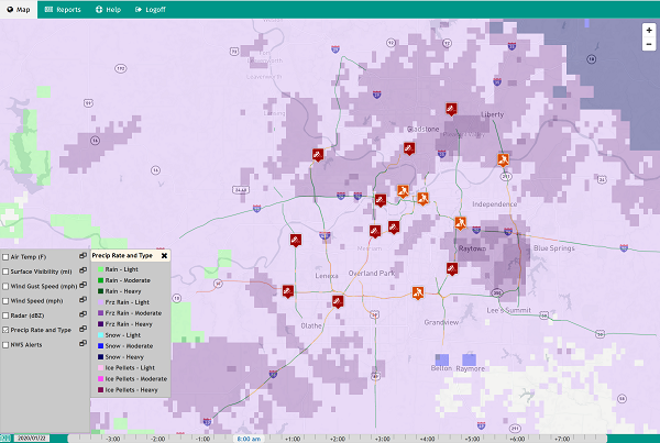

The figure depicts the IMRCP map interface with traffic, incident, and weather conditions during a major winter storm across the Kansas City region on January 22, 2020. Light purple indicates light frozen rain across most of the region, while pockeds of moderate and heavy frozen rain are scattered throughout the map in darker purple. Icons indicating roadwork and road conditions are scattered along the major roadways, which indicate traffic flow by green, yellow, and red.

Figure 2. Screenshot. User interface of an example map in the Integrated Modeling for Road Condition Prediction system.
Source: Federal Highway Administration

Study Area Description and Modeling

The IMRCP phase 2 study area was selected from among several candidate locations in the United States to demonstrate a broad range of capabilities. The Kansas City region is subject to highly variable weather conditions, typical urban congestion patterns, and interesting hydrological characteristics. The specific study area within the metro area was chosen based on a combination of characteristics, including congested traffic, alternative routes, weather sensors, and hydrologically challenging areas (several streams are subject to severe flooding within the study area). A planning model for the city, available from the Mid-America Regional Council (MARC) metropolitan planning organization (MPO), was used as a basis for the phase 2 road network model.

KC Scout operator feedback in phase 2 indicated the IMRCP model needed to cover the entire metropolitan area to support TMC-based operations. KC Scout operators are accountable to the entire metro area and wanted a view of regional traffic and weather conditions rather than just a preselected subnetwork. As shown in figure 3, the IMRCP phase 3 study area greatly extends the phase 2 model (shown in red) to include all of the freeways monitored by KC Scout. Traffic modeling on the extended freeway network is provided by MLP. The TrEPS dynamic traffic assignment (DTA) model continues to be deployed in phase 3 only on the phase 2 freeway and arterial network.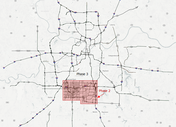

Map shows the greater Kansas City area, with Phase 3 major roads highlighted in black. Phase 2 is highlighted in red, and shows a small section on the southern end of the city, with a more intricate system of roads highlighted in black.

Figure 3. Map. Kansas City metropolitan study area of the Integrated Modeling for Road Condition Prediction.
Source: Federal Highway Administration; OpenStreetMap® contributors

This extension greatly increases the number of data sources for traffic, weather, and hydrology data. The phase 3 study area is made up of 5,936 roadway model links, 1,892 nodes, and 928 bridges. Data in the study area are collected from 205 traffic signals, 670 traffic detectors on the mainline freeway links, 332 ramp detectors, 178 StormWatch hydrological observing sites, 25 AHPS stations, and a NOAA Automated Surface Observing System (ASOS) station.

KC Scout is the primary operational stakeholder for the IMRCP demonstration deployment. Staff from KC Scout TMC, Missouri Department of Transportation (MODOT), and Kansas Department of Transportation (KDOT) supported the modeling effort and provided evaluation input for IMRCP after it was deployed. Real-time and archive data for the highway network were provided through KC Scout's TransSuite® data portals. Incident and work zone data were collected from KC Scout's event feed once per min, and traffic detector data consisting of speed, volume, and lane occupancy were collected from KC Scout's detector feed, also once per min.

Weather and hydrological data for the study area were gathered primarily from the NOAA sources described earlier but were supplemented with local sources such as the StormWatch system operated by the City of Overland Park, Kansas. Atmospheric weather forecasts are updated and retrieved once per hour. Hydrological systems generally update their data feeds only when the data change, but the IMRCP is configured to check those feeds at least once every 10 min to capture potential flash-flooding events. Based on these data availabilities, METRo road weather condition forecasts are recomputed once per hour. Weather conditions are provided with the 1-min traffic data updates to the TrEPS and MLP traffic models, which then recompute 2-h traffic condition forecasts once every 15 min.

Traffic Estimation and Prediction System Traffic Model

Calibration of the TrEPS traffic model is a critical and significant component of the integrated model deployment. This section summarizes the results of the model calibration effort. It provides a comparison between the model estimation results and the corresponding real-world observations.

Traffic Flow Model

The primary sources of traffic information were radar-based detectors installed along each of the three freeways (i.e., Interstate 435 [I–435], U.S. Route 69 [US–69], and Interstate 49 [I–49]) in the TrEPS study area (figure 4). Initial traffic flow model calibration was based on the 2018–2019 archived detector data provided by KC Scout. Detector-retrieved traffic parameters—including volume, speed, and occupancy—defined freeway traffic conditions in 1-min intervals. The daily 24-h traffic flow demand profile was described in a vector, which included 288 intervals of 5 min each of flow volume, speed, and occupancy. One-min aggregated values were used to estimate link-level speed-density relationships for each available detector.

Due to reliability, consistency, and availability issues, 69 detectors were adopted for the traffic flow model calibration. The archived data used to verify the relationship between speed and density consisted of 5- and 1-min aggregated historical detector data collected during 2017. Speed-density relationships were calibrated using the time-varying traffic data records: density and speed at 5-min measurement intervals. A two-regime traffic flow model form is used for traffic flow on freeways, while a single regime model form is used for arterials. Traffic flow model parameters include breakpoint density (k_bp), speed-intercept (v_f), minimum speed (v₀), jam density (k_jam), and the shape parameter (α).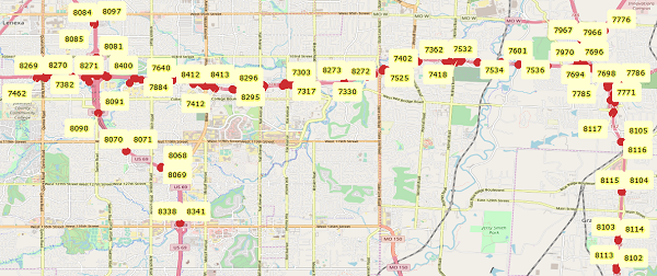

Figure 4. Map. Selected detectors for traffic flow model calibration by identifier code.
Source: Federal Highway Administration; OpenStreetMap® contributors

Freeway traffic flow models were divided into sections, depending on the freeway type of facility (i.e., mainline, on-ramp, off-ramp, or freeway-to-freeway ramp), direction of traffic, and free-flow speed characteristics. The calibrated speed-density curves for the network are documented in the Integrated Modeling for Road Condition Prediction [Phase 2] Final Report.⁵ The graphs therein represent typical example freeway links for which the observations were available, grouped by type of section they belong to.

Weather Adjustment Factors

Relevant literature findings^6,7 have shown that the traffic flow model parameters—the maximum service flow rate (qmax), shape parameter (α), and free-flow speed (uf)—are sensitive to both rain and snow intensities. As the rain or snow intensity increases, maximum flow rate, speed intercept, and free-flow speed are reduced.

A historical weather data set obtained from KC Scout and NWS sources from May to December, 2016, provided sufficient detail relative to visibility and precipitation intensity levels for calibration. However, since heavy rain and snow conditions appeared very rarely (i.e., were not recorded in the archived data set with great enough detail for weather adjustment factors [WAF] to be calibrated), the detectors did not provide enough data for traffic flow model calibration for heavy rain and snow weather conditions. Lack of adverse weather data within the archived data set, particularly a representative number of rain and snow days with associated parameters, coupled with the necessity of examining the traffic model's prediction quality for adverse weather conditions motivated the use of previously-calibrated WAF from a greater Chicago area network.⁸

Online Traffic Flow Model Update

The parameters of the traffic flow models embedded in the TrEPS platform are considered to be random variables with probability distribution due to inherent stochasticity of traffic behavior associated with flow breakdown during congested periods. This distribution can be shifted by external factors such as weather, variable speed limits (VSL), and nearby roadworks. To capture this time-variant traffic behavior, TrEPS updates the parameters of the traffic flow models online. The update process is initiated by speed deviation between predicted and observed detector values, which is continuously monitored in the consistency checking module. If a speed deviation on an observed link exceeds a predefined threshold, the traffic flow model assigned to the specific link is updated with the most recent detector data extracted from the IMRCP server. In adverse weather, the weather-adjusted traffic flow model is updated by adjusting the parameters of the base traffic flow model while pre-calibrated WAF remain intact.

Time-Dependent Origin-Destination Matrix

Joint estimation of the entire 24-h time-dependent origin-destination (TDOD) demand pattern was used in this study. Most previous DTA applications are limited to estimating peak-period demands. The 24-h demand was generated by extrapolating the estimated origin-destination (OD) demand from the peak period to an overall daily pattern. The static/historical demand matrix retrieved from the 2010 MARC transportation planning model, along with time-dependent traffic counts on selected observation links, was used to develop TDOD matrices over the time horizon with a chosen time interval (5 min).

The static/historical OD demand matrix for the Kansas City subnetwork was retrieved from a much larger 2010 MARC transportation planning model, which consisted of 981 zones and was developed for a peak period. To estimate the demand, the study area subnetwork (69 zones) demand was first extracted and then calibrated based on the detector data available.

For the OD extraction for the subarea under study, four types of trips relative to the subarea were observed: Internal–Internal (I–I), External–Internal (E–I), Internal–External (I–E), and External–External (E–E). I–I trips could be easily extracted from the original OD matrix. However, the effects of E–I and I–E on the subarea network also needed to be considered. To do so, a simulation of the entire network in Network EXplorer for Traffic Analysis (NeXTA) had been performed to retrieve vehicles' trajectory, and the number of vehicles entering or exiting the subarea had been added to the I–I trips with their corresponding zones. After the procedure was completed, total demand for the subarea was 1,438,515 trips per day.

Offline Calibration of the Origin-Destination Matrix

The demand extracted in the previous section needed to be calibrated based on the archived detector data. This section discusses the detector data, demand calibration, and the results.

Data Sources

The time-dependent link counts on selected observation links within the Kansas City phase 2 network were used with DTA models for calibrating time-dependent OD matrix. The characteristics of traffic count data used in this project are shown in Table 1. Out of 148 detectors available in archive data, 79 were excluded for reasons such as unreliable daily counts, inconsistencies in mass balance, or uncharacteristic speed-density relationships. The remaining 69 detectors were used for offline demand calibration.

Demand Calibration

The demand calibration was based on minimizing the weighted distance between historical OD and detectors values, with weights of w and (1−w), respectively. Additionally, time weights and links weights were devised to impose more control over time and individual link calibration.

In each DTA simulation, a number of iterations of the user equilibrium algorithm were applied to reach an equilibrium state in the network. Initially, a sensitivity analysis on parameter w was conducted to select the optimal weights in the objective function corresponding to the deviation from historical demand and link counts. The sensitivity analysis includes two ranges of values for parameter w. The first range includes 0.1–0.9, with increments of 0.1, for the deviation from historical demand. The second range includes the following values: 0.99, 0.999, and 0.9999.

Figure 5 shows deviations from observations and the deviation from the target demand under different weight selections in the first iteration of the basic solution method. By comparison, w = 0.9 gives a decent compromise between two deviation terms in the objective function and is selected for numerical experiments. The link weights have been carefully selected so the simulation better matches the observation. The time weights of the 288 intervals (total of 24 h) of demand may vary from period to period.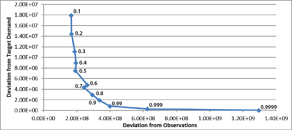

Graph shows deviation from target demand on the Y axis from 0.00E+00 to 2.00E+07, and deviation from observations on the x axis from 0.00E+00 to 1.40E+09. At 2.00E+08 deviation from observations, the line is at 0.1, then sharply falls to 0.99 by 4.00E+08 deviation from observations. The line then slowly decreases the rest of the graph, until hitting 0.9999 near 1.40E+09.

Figure 5. Graph. Sensitivity analysis of different weights.
Source: Federal Highway Administration

Calibration Results Evaluation/Validation

The TDOD estimation was first validated on a link-level basis, and then the overall calibration results, including the traffic flow model, WAF, and TDOD, were taken into DYNASMART-X and verified by the comparison between simulation data and historical observation data.

First, the simulated and observed link counts are compared for each link. Simulation results based on the estimated time-dependent OD matrix are compared with the actual observations. Results showing the 5-min and cumulative vehicle counts for three selected links before and after calibration are documented in the Integrated Modeling for Road Condition Prediction [Phase 2] Final Report.⁹ The graphs therein represent typical example freeway links for which the observations were available, grouped by type of section they belong to.

Online Calibration of the Origin-Destination Matrix

Due to the variety of weather patterns, lack of data, and the time-consuming calibration process, it is not feasible to prepare demand input in regard of all possible weather situations. In IMRCP phase 3, the research team modified the OD demand estimation/prediction module in TrEPS to combine the knowledge learned from correlation analysis between weather factors and observed traffic volume into an online demand estimation and prediction framework. Two levels of weather-sensitive demand adjustment are considered in this framework: (1) the weather-affected demand factors can reflect the network-wide demand reduction into a priori demand, while (2) the regional difference of weather impact would be addressed in a demand estimation/prediction module that executes zonal demand adjustment based on traffic states discrepancy between link traffic measurement and simulated link traffic states. The framework of online traffic demand calibration in TrEPS is shown in figure 6.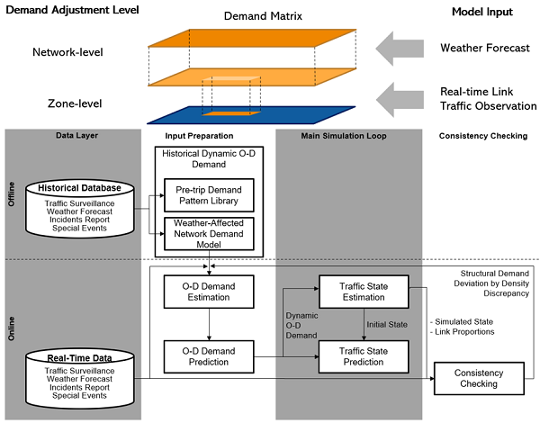

THe Model Input includes Weather Forecast and Real-time Link Traffic Observation, which lead into the Demand Matrix, which includes the Demand Adjustment Level, Network-level and Zone-level. Offline, the Data Layer includes historical database, which includes traffic surveillance, weather forecast, incidents report, and special events. That leads to the input preparation Historical Dynamic O-D Demand, which includes pre-trip demand pattern library and weather-affected network demand model. Online, the data layer real-time data includes traffic surveillance, weather forecast, incidents report, and special events. Real-time data and historical dynamic O-D demand lead to online input preparation O-D Demand Estimation, which leads to O-D Demand Prediction. Through dynamic O-D demand, the main simulator loop includes traffic state estimation and traffic state prediction, connected by Initial State. Traffic State Estimation, through simulated State and Link Proportions, goes to consistency checking. Through Structural Demand Deviation by Density Discrepancy, the loop goes back to the input preparation.

OD = origin-destination

Figure 6. Diagram. Framework of online traffic demand calibration in Traffic Estimation and Prediction System.
Source: Federal Highway Administration

Machine Learning-Based Traffic Prediction

The MLP package predicts traffic network conditions given a set of system variables including weather, work zones, incidents, and special events. MLP is a comprehensive data-driven prediction module and considers a Markov process to explicitly characterize the probabilistic transition between traffic states under different external conditions (e.g., weather, incidents). It is able to accurately capture the recurring and non-recurring traffic congestion. MLP provides a reliable prediction of traffic speeds for traffic management centers to efficiently deploy proactive traffic management strategies.

Model

The MLP package contains three classes: MLP scenario identifier, MLP traffic predictor, and MLP update manager.

The scenario identifier identifies what specific scenario the current traffic condition belongs to and then selects/generates corresponding models for traffic state prediction. It contains three parts: a traffic state cluster, a Markov model generator, and a decision tree model. All three parts use the archived data as input and provide established models for the future use. The traffic state cluster defines the traffic states based on the levels of traffic speeds. The Markov model is developed based on historical traffic state transitions and is used to explain the stochastic evolutions of traffic states for each link. The decision tree model identifies the conditions regarding whether a certain external event will influence the traffic condition.

The traffic predictor predicts likely future network traffic states for a specified prediction horizon (such as 15 min, 30 min, 1 h, or 2 h) under specific network external conditions. The traffic predictor uses information on current network link traffic states and other system variables, such as work zones and incidents, as model inputs to predict future network states. The traffic predictor considers different transition probabilities between traffic states under different external conditions (e.g., weather, incident) and uses a time series model to account for the latest trends and observations from the field. Therefore, it is able to accurately predict traffic state evolution under different external conditions and can adjust the prediction based on real-time field observations.

The update manager is built as a part of the prediction process that maintains and updates the latest MLP parameters. The purpose of the online update is to use both the empirical and real-time distribution of travel speed/time for different traffic conditions to enhance prediction accuracy and robustness. The update manager has two tasks. First, it updates the distribution of key traffic variables using the updated data store (e.g., traffic speed, volume) and prepares them for use by the traffic predictor. Second, it schedules periodic updates to the traffic predictor through a recalibration process using new data collected from the previous period.

To be specific, figure 7 illustrates the main components of the MLP models. The algorithm considers that the environment variables (e.g., weather) and external event variables (e.g., incidents) affect the transition probability matrices between different traffic states. A decision tree model based on the historical data determines if the external events are influential to the traffic condition and whether the Markov model will be applied. The time series model takes online data as input to reflect the most current traffic conditions observed in the field. This makes the prediction model robust, particularly during special conditions that have different traffic patterns from regular scenarios.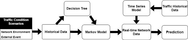

Traffic Condition Scenarios start with network environment external event, leading to historical data, leading to decision tree. Historical Data and decision tree both lead to markov model, leading to real-time network data, leading to prediction. Traffic historical data also leads to time series model which also leads to real-time network data.

Figure 7. Diagram. Proposed machine learning-based prediction model algorithm.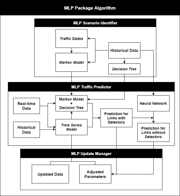
Source: Federal Highway Administration

MLP Package Algorithm starts with MLP Scenario Identifier. Historical data leads to traffic states, which leads to markov model, and decision tree. MLP traffic predictor is the next grouping. Historical data leads to neural network, which leads to prediction for links without detectors. Decision tree and Markov model lead to markov model and decision tree. Real time data also leads into markov model and decision tree. Histoircal data leads to time series model, which also leads to markov model and decision tree, which all lead to prediction for links with detectors. The last grouping, MLP Update Manager, has Time Series Model leading to both updated data and adjusted parameters, and prediction for links with and without detectors leading to adjusted parameters.

Figure 8. Diagram. Representation of the Integrated Modeling for Road Condition Prediction machine learning-based prediction (MLP) process.
Source: Federal Highway Administration

Data

A total of 14 variables are categorized into three groups, including network environment, external event, and traffic states. The traffic states are collected by detectors and the weather data are collected from NWS modeling and forecast systems for use within the IMRCP system.

Model Calibration

Figure 8 shows a graphical representation of the IMRCP MLP algorithmic flow. First, MLP understands which facility group (e.g., functional type) the link belongs to and extracts data about network external condition scenarios (e.g., system variables, such as weather and incidents). Then, it pulls the most relevant historical data and calculates inputs for the Markov and time series models. Online detector data feeds are also used as inputs to ensure predicted traffic conditions can best reflect real-time conditions. In the MLP software, to predict traffic for links without detectors, a neural network model is constructed by fusing data of different sources (i.e., detector observation and real-time prediction data from nearby links). Predicted values from the nearest downstream links with detectors (within 10 miles) for normal conditions are used for the prediction of links without online data. This extends the predictability of most of the links on the network. For remote links without detectors nearby, it is recommended to use either online or historical private sector data (e.g., INRIX, HERE) for prediction.

Results

The prediction results of the normal case are shown in figure 9; cases with incidents are shown in figure 10. The Markov-based model is compared with a weighted time series model without Markov processes. Figure 11 shows the predictions of light and heavy rain conditions and light and heavy snow conditions. For all cases, the model can capture the drops and turning-backs well.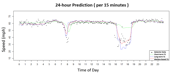

Graph shows speed by mph on the y-axis and time of day from 0 to 23 on the y-axis. lines show short-term TS, long-term TS, and markov-based TS, and points show detector data. Speed stays around 60 mph at all hours of the day except for the dip at 8 down to 40 mph and from 16 to 19, where long-term TSM and Markov-based TS dip to around 30 mph, and short-term TS dips to around 50 mph.

mph = miles per hour. TS = time series.

Figure 9. Graph. Prediction of normal case with daily traffic patterns.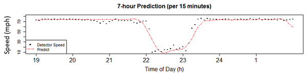
Source: Federal Highway Administration

Graph shows 7-hour prediction with speed from 10 to 80 mph on the y-axis and time of day from 19 to 2 on the x-axis. Predict is shown by a dotted line and detector speed is shown by dots. both detector speed and predict stay at 70 mph except for the dip between 22 and 24, where predict and detector speed drop to 10 mph.

A. Graph. Predictions of speeds with incident (per 15 minutes).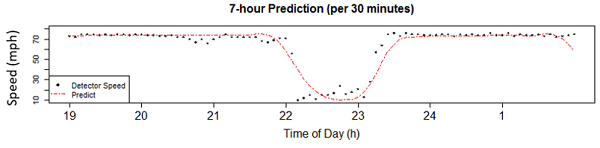

Graph shows 7-hour prediction with speed from 10 to 80 mph on the y-axis and time of day from 19 to 2 on the x-axis. Predict is shown by a dotted line and detector speed is shown by dots. both detector speed and predict stay at 70 mph except for the dip between 22 and 24, where predict and detector speed drop to 10 mph.

B. Graph. Predictions of speeds with incident (per 30 minutes).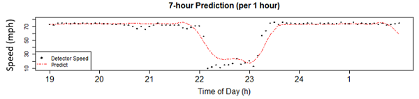

Graph shows 7-hour prediction with speed from 10 to 80 mph on the y-axis and time of day from 19 to 2 on the x-axis. Predict is shown by a dotted line and detector speed is shown by dots. both detector speed and predict stay at 70 mph except for the dip between 22 and 24, where predict and detector speed drop to 10 mph.

C. Graph. Predictions of speeds with incident (per 1 hour).

h = hour. mph = miles per hour.

Figure 10. Graphs. Predictions of speeds with incident on link.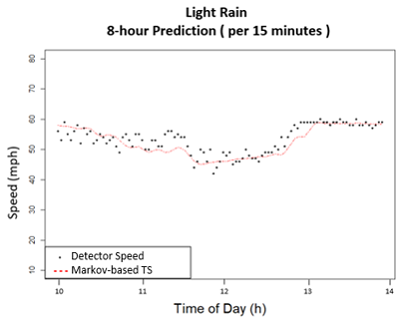
Source: Federal Highway Administration

Graph shows 8-hour predictions per 15 minutes in light rain, with speed in mph from 10 to 80 on the Y-axis and time of day in h from 10 to 14 on the X-axis. Detector Speed is shown in black dots and Markov-based TS is shown in red dotted lines. Speed starts around 60 mph at 10, slowly declines to about 45 mph at 12, then quickly climbs back up to 60 mph by 13 and 14.

A. Graph. Speed Predictions (Light Rain).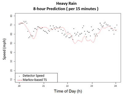

Graph shows 8-hour predictions per 15 minutes in heavy rain, with speed in mph from 10 to 80 on the Y-axis and time of day in h from 20 to 24 on the X-axis. Detector Speed is shown in black dots and Markov-based TS is shown in red dotted lines. Speed starts around 70 mph at 20 h, but quickly drops to 55 before 21 h, then goes back up to 65 by 21 h. Speed holds around 65 until 22 h, when it drops to 50 mph, and fluctuates between 50 mph and 60 mph until 23 h, when speed jumps back up to 65 mph by 24 h.

B. Graph. Speed Predictions (Heavy Rain).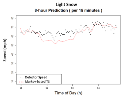

Graph shows 8-hour predictions per 15 minutes in light snow, with speed in mph from 10 to 80 on the Y-axis and time of day in h from 11 to 14 on the X-axis. Detector Speed is shown in black dots and Markov-based TS is shown in red dotted lines. Speed starts around 70 mph at 11 h and slowly declines to 50 by 12.5 h, then climbs back up to 70 mph by 14 h.

C. Graph. Speed Predictions (Light Snow).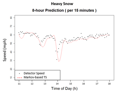

Graph shows 8-hour predictions per 15 minutes in heavy snow, with speed in mph from 10 to 80 on the Y-axis and time of day in h from 11 to 18 on the X-axis. Detector Speed is shown in black dots and Markov-based TS is shown in red dotted lines. Speed starts around 60 mph at 11 h, and between 12 and 13 h drops to 45 mph. Speed slightly increases to 60 mph by 14 h but then heavily drops to 30 mph. By 15 h, speed is back up to 50 mph, and has a slow constant increase until 18 h at 60 mph.

D. Graph. Speed Predictions (Heavy Snow).

h = hour. mph = mile per hour. TS = time series.

Figure 11. Graphs. Predictions of speeds with rain and snow weather condition.
Source: Federal Highway Administration

Error rates, root mean square error, and mean absolute error are used to evaluate the performance of the proposed model. The error rates of the normal case are between 5 and 9 percent. For the cases with an incident on the link or downstream of the link, the error rates of the predictions for the Markov-based model are between 9 and 18 percent, while the error rates of the time series model, without the Markov process, is between 53 and 60 percent. It shows that the MLP package using the Markov-based time series model is significantly more accurate than the traditional time series model. The prediction of weather events shows that the model can generally capture the drops and trends of speeds during the weather conditions. The error rates are below 10 percent and the root mean square errors are below 6 percent.

Predictions of special events are conducted. Links are selected based on the observation of historical data sets. Examples for game days of the Kansas City Royals are shown in figure 12. Generally, the predictions of the model can capture the congestion patterns caused by special events well.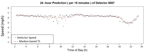

Graph shows 24-hour prediction per 15 minutes of Detector 8007. Speed in mph from 10 to 80 is on the Y-axis and time of day in h from 2 to 24 is on the X-axis. Detector Speed is shown in black dots and Markov-based TS is shown in red dashed line. Both lines generally correlate together on the graph. Speed holds steady at 65 mph from 2 h to around 8 h, when there's a slight decline to 60 mph by 10 h. Speed then increases slowly to 70 mph by 12 h, and holds steady until about 20 h, when speed declines to 55 mph by 22 h, then increases again to 65 mph by 24 h.

h = hour. mph = mile per hour. TS = time series.

Figure 12. Graph. Examples of predictions for special events.
Source: Federal Highway Administration

For links with no detectors providing real-time traffic data, data from the downstream detectors will be utilized to predict the future speed values. A neural network model is built to predict the link traffic speed under normal cases based on the downstream detector data. If there are external conditions, the same transition matrices are applied. Predictions of traffic speed during 10 days on two detectors are show in figure 13. The predicted values can detect recurrent patterns and speed drops, including congestions caused by incidents. The error rates are about 3.5 percent and 2 percent, which are satisfactory.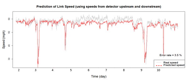

Graph shows Prediction of Link Speed using speeds from detector upstream and downstream. Speed in mph from 30 to 60 is on the Y-axis, and time from 2 to 10 is on the X-axis. Real speed is shown in grey while predicted speed is shown in red. Throughout the graph, real speed and predicted speed follow the same pattern, though real speed is a few mph higher than predicted speed. Speed starts around 57 mph at 2, then drops to 20 mph at 3, then jumps back up to 55 mph right after 3. Right before 5, there's another drop to 40 mph, then speed goes back up to 55 mph. Speed holds around 50 to 55 mph until 9, when speed drops to 30 mph, and again at 10, when speed again drops from 55 mph to 30 mph. The error rate is 3.5 percent.

A. Graph. Predictions for detector with incidents.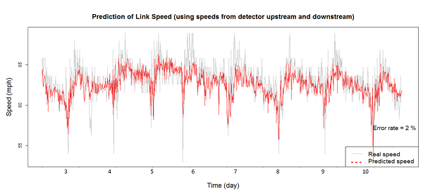

Graph shows Prediction of Link Speed using speeds from detector upstream and downstream. Speed in mph from 55 to 65 is on the Y-axis, and time from 3 to 10 is on the X-axis. Real speed is shown in grey while predicted speed is shown in red. Throughout the graph, real speed and predicted speed follow the same pattern, though real speed has higher and lower speeds when the predictions peak. Speed follows a cycle that starts off faster at the top of the hour, near 65 mph, and drops at the bottom of the hour, near 55 mph, following the same cycle each hour. The error rate is 2 percent.

B. Graph. Predictions for detector with recurrent patterns.

mph = mile per hour.

Figure 13. Graphs. Examples of predictions for links without detectors.
Source: Federal Highway Administration

Generally, the results show a relatively accurate prediction under the conditions of incidents and bad weather conditions, with error rates between 4 and 18 percent. Compared to the benchmark models, the MLP model can capture the most potential changes in traffic states and can provide a reliable prediction using the Markov transition matrices. The performance of the MLP package is superior to the benchmark model for both cases with and without external conditions. The MLP package is able to accurately capture the recurring and non-recurring traffic congestion.