Decision Support Framework and Parameters for Dynamic Part-Time Shoulder Use:
Considerations for Opening Freeway Shoulders for Travel as a Traffic Management Strategy
Chapter 4. Decision Parameters for Opening the Shoulder
This chapter describes methods for determining when the shoulder of a dynamic part-time shoulder use (D-PTSU) freeway should be opened to traffic. The traffic operations decision parameters for temporarily opening a shoulder to traffic will vary from facility to facility, and this chapter describes how an agency can go about determining the appropriate decision parameters and thresholds for opening the shoulder.
The methodology to determine the appropriate conditions for opening the shoulder and the operational decision parameters should consider the following:
- Variations in capacity—roadway capacity is not a fixed value and changes based on vehicle speeds, vehicle mix, driver population, and environmental conditions.
- The time required to initiate and complete the shoulder opening process (i.e., the sweep time).
- The rate of increase in the traffic flows leading up to the peak period.
- The geometry of the specific facility, such as grades and heavy merges, diverges, or weaving.
- The extent to which these thresholds will vary with time of day, day of week, time of the year, weather conditions, and the combination of all these conditions.
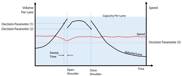
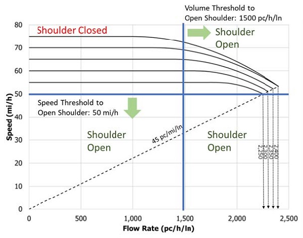
Figure 13 illustrates the application of an agency's speed and volume thresholds, generally developed in a concept of operations (ConOps) document, to determine when to open and close the shoulder lane during a typical peak period. In this example, the agency has a volume threshold (decision parameter 1) and a speed threshold (decision parameter 3) to open the shoulder. A second, lower volume threshold, decision parameter 2, exists for closing the shoulder. In reality, both the opening and closing decision parameters could also be functions of speed and volume combinations rather than each of these in isolation as shown in this example.
Source: FHWA
Figure 13. Diagram. Example application of speed and volume decision parameters.
In this example the volume threshold to open the shoulder is initiated first, before the speed threshold. Different values and a different speed-flow relationship for the freeway could have resulted in the reverse condition.
There is a delay—the sweep time—between the times when the threshold to open the shoulder is reached (decision parameter 1) and when the shoulder is opened to traffic. This is the time required for the shoulder to be inspected to verify it is free of debris and disabled vehicles. The sweep time is also used to notify stakeholders such as law enforcement that the shoulder will be opening. Thus, a decision parameter ideally anticipates the actual onset of congestion. In this example, decision parameter 1 is well below the capacity.
The volume per lane drops suddenly when the shoulder is opened because the same flow divided by more lanes results in a drop in volume per lane. The volume per lane then jumps suddenly when the shoulder is closed. The closing threshold volume (decision parameter 2) is set low enough that the shoulder closure does not suddenly cause new congestion in the remaining lanes. This is why it is desirable to have a slightly lower volume threshold (decision parameter 2) for closing the shoulder than for opening it.
Since opening the shoulder in this example prevents the onset of significant congestion, a speed threshold for closing the shoulder would not apply (the speed recovers rapidly after the shoulder is opened, after which the speed does not provide a useful indication of when the shoulder can be closed). Consequently, the volume threshold (decision parameter 2) is used to determine when the shoulder can be closed without inadvertently creating congestion on the freeway.
Methods for Selecting Shoulder Use Type and Decision Parameters
Five data-driven methods exist for selecting and optimizing the opening time of a D-PTSU facility. While they are primarily presented in this chapter in the context of making decisions day-to-day, they could also be used during ConOps development to establish hours of operations for static part-time shoulder use (S-PTSU) or core hours of operations for D-PTSU. Some methods are more applicable to day-to-day use, and others are more applicable to use at the ConOps stage. The five basic methods include:
- Demand-to-Capacity Patterns — Using sensors or traffic counts on the facility, an operating agency assesses historical demand profiles to determine levels of congestion relative to the available facility base capacity as well as the expected capacity with shoulder use.
- Empirical Performance Data — Using whole-year travel time reliability data, an operating agency explores the frequency and pattern of breakdown events to identify times when the facility experiences congestion.
- Macroscopic Decision Parameter Optimization — Using the Highway Capacity Manual (HCM) freeway facilities method, an operating agency examines different types of decision parameters (speed vs. volume-based) and decision parameter values for a facility. It does this using an iterative approach to determine the optimum decision parameter for the facility, a process that can be automated through software.
- Microscopic Decision Parameter Refinement — Using calibrated microsimulation tools, an operating agency simulates the facility in question with the initial proposed decision parameter algorithm. It uses the simulation assessment to verify the concepts developed through the macroscopic optimization, which can be refined for the facility-specific geometry and traffic patterns.
- Monitoring and Adjustment — On a Level 3 or Level 4 D-PTSU facility, which are defined as a dynamic PTSU with core hours and unscheduled variation and a fully dynamic PTSU, respectively, the operating agency uses realtime operating experience to adjust the decision parameter values and open or close the shoulder at different thresholds. By monitoring shoulder operations for the first few weeks after implementation of the thresholds, the operator adjusts the thresholds and decision parameters as necessary to meet the agency's objectives for operating the facility. Monitoring should be continued but can be less intensive once the operator has acquired experience with the operations of D-PTSU.
The details of these methods are described later in this chapter, after linking the methods to specific use cases and analysis questions in the following section.
Use Cases for Shoulder Use and Decision Parameter Selection
The selection and adequacy of the aforementioned methods is a function of the intended goals of the agency or operator. Three common use cases are introduced below that represent frequent questions an agency may have related to PTSU:
- Would D-PTSU be an appropriate strategy in a location where no PTSU (even static) is currently in place?
- Should D-PTSU be considered in a location where S-PTSU is in place?
- How can an agency better optimize the operations of an existing D-PTSU installation?
For each use case, one or more of the methods are used to inform agency decisionmaking.
Would Dynamic Part-Time Shoulder Use be an Appropriate Strategy in a Location Where No Part-Time Shoulder Use (Even Static) Is Currently in Place?
An agency exploring the use of D-PTSU on a facility needs first to develop an understanding of congestion patterns on the facility (spatial and temporal extents of congestion) as well as the underlying causes of congestion. This use case is best approached with a combination Method I — Demand-to-Capacity Patterns and Method II — Empirical Performance Data.
To explore the viability of D-PTSU, an agency can look at demand-to-capacity (d/c) ratios, including fluctuations in d/c ratios. From this, d/c combinations where PTSU is most effective, which are typically shorter periods of congestion, can be identified.
Combining d/c analysis with an investigation of empirical performance data identifies the distribution of breakdowns across days of week and time of day, and determines when a dynamic system may provide benefit over a static system.
That said, many agencies are choosing to skip static part-time shoulder use (S-PTSU) and are starting at a Level 2 D-PTSU system or above. This provides flexibility in dealing with incidents, inclement weather, and planned special events.
Should Dynamic Part-Time Shoulder Use Be Considered in a Location Where Static Part-Time Shoulder Use Is in Place?
Similar to the previous use case, this question is best approached with a combination of Method I — Demand-to-Capacity Patterns and Method II — Empirical Performance Data. The applicability of S-PTSU versus D-PTSU is a function of the distribution of breakdown events. Are periods of high d/c ratios uniformly distributed and predictable, or scattered across the day, on weekends, and as a function of seasonal variability? An S-PTSU system may be a reasonable choice when congestion is highly predictable (e.g., 7–9 a.m. every weekday), while a D-PTSU system applies when congestion patterns are more random. A reliability analysis (Method II) helps in this assessment: the less reliable a facility, the more useful it is to move towards a dynamic system.
A related question is whether the operating hours of an S-PTSU system should be expanded (vs. migrating to D-PTSU). This question can similarly be answered using Methods I and II. If analysis finds that high d/c ratios and congestion that once occurred from 7–9 a.m. now extend until 10 a.m., then increasing the hours operations is a viable approach—assuming no other changes in the reliability of the system.
How Can an Agency Better Optimize the Operations of an Existing Dynamic Part-Time Shoulder Use Installation?
To answer this question, the three more advanced methods (Method III, IV, and V) are used to augment the analysis from Method I and II. A thorough understanding of congestion patterns and temporal and spatial distributions of congestion is still the starting point.
Once an agency decides to implement D-PTSU, Method III: Macoscopic Decision Parameter Optimization can be used to develop guidance on when to use volume-based versus speed-based decision parameters. Each has benefits and tradeoffs, which are described in the discussion of Method III below.
Method III can be based on a generic facility, which is how it is described in the discussion of Method III below for the purposes of this report. However, for a specific D-PTSU project, the method can be customized to replicate the specific geometry and demand patterns of the subject facility. As such, the FREEVAL method, which will be introduced in the discussion of Method III, can be used to model a specific facility. FREEVAL uses underlying algorithms to quickly and efficiently test different decision parameter combinations.
With the macroscopic results and a set of facility-specific decision parameters in place, an agency may chose to conduct a microsimulation analysis (Method IV: Microscopic Decision Parameter Refinement) to verify the effects. An example for this is illustrated in the discussion of that method later in this chapter.
Finally, Method V: Monitoring and Adjustment applies to existing facilities, with operators monitoring day-to-day operations of the D-PTSU system and making adjustments based on observed congestion patterns.
Bottleneck Identification
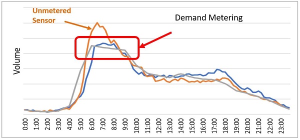
A key component of PTSU decisionmaking, regardless of the method used for determining decision parameters, is locating and understanding bottlenecks. In the experiments conducted as part of this report, bottlenecks were modeled as on ramps, but other freeway features such as uphill grades, bridges, tunnels, or lane drops could also be bottlenecks. In recent years, probe data sources provided by commercial vendors have become popular tools for identifying bottlenecks. However, sensors are needed to measure the capacity of bottlenecks and the demand, so sensor placement is key. Sensors may not measure the true demand if they are located downstream of an active bottleneck or within a queued segment, and should be located right at a bottleneck for accurate measurement of demand and capacity. Sensors that are impacted by congestion in these ways will only measure the throughput or "volume served" as opposed to the true demand. To avoid this metering effect, the selected sensor should be upstream of congestion and free of any queuing patterns. Alternatively, an unconstrained demand profile can be used to estimate demand from the known daily volumes in the bottleneck. To illustrate this point, figure 14 shows an example of two metered sensors as well as one unconstrained sensor from a congested freeway. While all three sensors have the same demand over a 24-hour period (same facility), the measured volume profiles plateau for the two sensors impacted by congestion.
Source: FHWA
Figure 14. Chart. Example of freeway sensor metering due to congestion.
Method I: Demand-to-Capacity Patterns
The first step towards implementing or improving PTSU is to develop an understanding of d/c patterns. Congestion on freeways is caused by demand exceeding capacity, with unserved demand translating into a queue and congestion. For recurring congestion, it is common that (fixed) capacity at a bottleneck is exceeded by surges in demand during certain times of day. These time periods are generally good candidates for a (part-time) capacity enhancement treatment such as PTSU.
Alternatively, the d/c ratio may also exceed 1.0 when the denominator—the capacity—is temporarily reduced due to weather, an incident, a work zone, or other similar events. In these non-recurring congestion cases, PTSU is less likely to be applicable, given that the underlying reason capacity is compromised (incident, weather, etc.) is likely to affect the shoulder also.
In designing a PTSU system, agencies need to understand how high the true demand is relative to the available capacity. In the HCM, the "ideal" capacity of a basic freeway segment is 2,400 passenger cars per hour per lane (pc/h/ln) for a freeway with free-flow speed (FFS) of 70 mi/h and above, with that capacity being reduced by 50 pc/h/ln for each 5 mi/h drop in FFS. However, in a freeway facility context, the HCM also recognizes bottleneck capacities are often significantly lower than the values in table 7.
| Location | No of Lanes | Average (Standard Deviation) | ||
|---|---|---|---|---|
| Breakdown {XE "Breakdown"} Flow | Maximum Prebreakdown Flow | Queue {XE "Queue"} Discharge Flow | ||
| Minneapolis, Minn. | 2 | 1,876 (218) | 2,181 (163) | 1,644 (96) |
| Portland, Ore. | 2 | 2,010 (246) | 2,238 (161) | 1,741 (146) |
| Toronto, Canada | 3 | 2,090 (247) | 2,330 (162) | 1,865 (124) |
| Sacramento, Calif. | 3 | 1,943 (199) | 2,174 (107) | 1,563 (142) |
| Sacramento, Calif. | 4 | 1,750 (256) | 2,018 (108) | 1,567(115) |
| San Diego, Calif. | 4 | 1,868 (160) | 2,075 (113) | 1,665 (85) |
| San Diego, Calif. | 5 | 1,774 (160) | 1,928 (70) | 1,600 (66) |
Source: Highway Capacity Manual, Sixth Edition. 2016. Exhibit 14-2, Transportation Research Board, Washington, DC.
Assuming a shoulder capacity of 1,600 passenger cars per hour (pc/h) and a freeway bottleneck capacity of 2,000–2,200 pc/h/ln, target d/c ratios for PTSU viability can be derived (table 8). Shoulder capacities vary greatly from facility to facility, and 1,600 pc/h is used here to represent a shoulder with a relatively high capacity that is still less than a general purpose lane. The table develops a blended cross-section capacity for a PTSU facility with two, three, or four general purpose lanes in one direction (not counting the shoulder). A comparison of this blended capacity with PTSU to the base capacity allows for the development of a target d/c ratio. If the demand profile of a facility stays below that target ratio (but exceeds 1.0 for parts of the day), PTSU may be a viable treatment.
| Base Number of Lanes | Base Capacity (pc/h/ln) | Capacity with PTSU added (pc/h/ln) | Ratio of PTSU vs. Base → PTSU d/c Ratio Target |
|---|---|---|---|
| 2 | 4,000–4,400 | 5,600–6,000 | 1.40 – 1.36 |
| 3 | 6,000–6,600 | 7,600–8,200 | 1.27 – 1.24 |
| 4 | 8,000–8,800 | 9,600–10,400 | 1.20 – 1.18 |
d/c = demand-to-capacity (ratio). pc/h/ln = passenger cars per hour per lane. PTSU = part-time shoulder use.
The table suggests that PTSU can increase capacity by 35–40 percent for a two-lane freeway, 25–30 percent for a three-lane freeway, and 15–20 percent for a four-lane freeway. For facilities (or time periods) with d/c ratios greater than 1.4, 1.3, or 1.2 for two-, three-, and four-lane facilities, respectively, a PTSU system will not provide sufficient added capacity to relieve congestion. PTSU facilities have been removed after 25–30 years of operation because they were no longer providing adequate capacity. I-95/SR 128 in Massachusetts was widened by one additional lane in each direction to provide additional capacity at off-peak times, and I-66 in Virginia is currently being widened to provide multiple additional lanes in each direction.
PTSU can increase capacity by 35–40 percent for a two-lane freeway, 25–30 percent for a three-lane freeway, and 15–20 percent for a four-lane freeway. For facilities with pre-PTSU demand to capacity ratios greater than 1.4, 1.3, or 1.2 for two-, three-, and four-lane freeways, respectively, PTSU will not add sufficient capacity to relieve congestion.
At the same time, it is important to recognize that for facilities with a d/c ratio of 1.05 or below, a PTSU system may not be necessary, as other transportation system management and operations strategies such as ramp metering may provide a better benefit-cost ratio at those low degrees of oversaturation.
In applying these concepts to a PTSU evaluation, an agency should ask the following questions:
- When (in time) does demand exceed capacity?
- Where (in space, which segments) does demand exceed capacity?
- How high is the demand relative to available capacity?
- How long does demand exceed capacity?
- How much do these patterns change from day to day?
An understanding of these questions for a given facility will help develop an understanding of the underlying causes of congestion and an initial hypothesis about the expected benefits of a S-PTSU or D-PTSU system.
Method II: Empirical Performance Data
The selection of decision parameter thresholds and the type of decision parameter starts with a thorough understanding of the congestion patterns on the facility. Since PTSU is primarily a congestion-relief treatment, the agency needs to understand where and when congestion typically occurs on a facility. It is further critical to distinguish between recurring congestion (repetitive congestion pattern due to capacity constraints relative to demands) and non-recurring congestion (variable congestion patterns due to volume fluctuations, weather, incidents, work zones, and seasonal effects). To some degree, this also determines the added benefits of D-PTSU over S-PTSU for a given facility.
To fully understand congestion patterns, it is desirable for an agency to evaluate congestion patterns for a period of at least 1 year of data, can be with agency collected data, probe data, or a combination of both. Archival probe-based data sources could come from the National Performance Monitoring Resource Data Set (NPMRDS), or a commercial data provider. Using one year of data, it is possible to derive congestion patterns and identify periods where PTSU may offer congestion relief.
Understanding congestion patterns further requires an assessment of the facility (bottleneck) capacity, and the level of demand relative to that capacity (see Method I). For this assessment, traffic sensors on the facility are used to gather speed/flow/density data at the bottleneck, which is then used to determine bottleneck capacities.
The empirical performance method consists of four steps:
- Assess Whole-Year Congestion — using archived data, determine congestion patterns, distinguish recurring and non-recurring congestion, and quantify temporal and spatial extents of congestion.
- Evaluate Breakdown Probabilities — from local sensor data, apply probability methods at the bottleneck to identify breakdown events and quantify breakdown flow rates (i.e., segment capacity).
- Explore Breakdown Distributions — use the results of the breakdown probability analysis to determine temporal distribution of breakdown events.
- Estimate Initial Decision Parameter Threshold — use whole-year speed-flow data and HCM capacity concepts to develop initial threshold values for speed- and volume-based decision parameters.
Assess Whole-Year Congestion
Analysis of a whole-year data set from sources like the NPMRDS provides insight about the temporal and spatial congestion patterns on a facility. The motivation for this analysis is to identify whether the congestion is recurring and predictable (e.g., every weekday morning from 7–9 a.m.), more random (e.g., sometimes breaks down in the afternoon, sometimes on the weekends), or some combination. In the context of identifying decision parameters, the more randomly the breakdown events are distributed, the more the decision parameter needs to be dynamic as opposed to static.
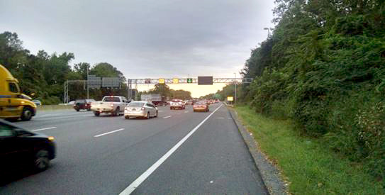
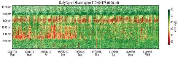
A whole-year speed and travel time dataset can be used to generate a heat map of corridor performance, which is used to understand congestion patterns. An example is given below for the eastbound portion of I-66 in northern Virginia, which was converted from a static (morning peak only) to a dynamic system in September 2015.1 The example includes a portion of I-66 upstream of the PTSU segment, the PTSU segment itself, and a portion of I-66 downstream of the PTSU segment. Figure 15 shows a photo of the facility, while figure 15 shows a representative heat map from one of the segments.
Source: Kittelson & Associates, Inc.
Figure 15. Photo. Gantry with dynamic lane use signs I-66 in Northern Virginia.
Source: Probe Data Analysis Tool: Summary of Case Studies
Figure 16. Chart. Speed heat map for eastbound I-66 analysis segment from probe data.
In figure 16, it is apparent that from September 2014 through around September 2015 there is heavy congestion during both the morning, midday, and afternoon hours. During the morning peak period, a S-PTSU system had already been in place. For the midday and afternoon peak hours, no PTSU was used, resulting in congestion on a subset of days. Since the congestion patterns in the midday and afternoon hours are not homogeneous, there is an indication that a dynamic system may provide some benefits (as opposed to just extending the S-PTSU operating hours). With the implementation of D-PTSU in September 2015, midday and afternoon peak congestion is notably reduced, while the morning peak period is unaffected. In a sense, the morning period acts as a control site for the effects of the D-PTSU system for other time periods.
Conversion of S-PTSU to D-PTSU on I-66 eastbound enabled the shoulder to be opened outside of the a.m. peak hour if the Virginia Department of Transportation desired. As a result, the average p.m. travel time for the eastbound PTSU segment decreased from 14.7 to 13.7 minutes, and the average weekend daytime travel time for the PTSU segment decreased from 14.5 to 13.1 minutes. Both results were statistically significant. (Suliman 2017)
In addition, the same probe data can be used to generate various visualizations on travel time reliability as well as to conduct a before-and-after analysis (once the system has been put in place, and to monitor operations). One example visualization is the "speed band" graphic shown in figure 17, which shows the average speed (red line) by time of day and the "reliability band" from the 5th to 95th percentile (shaded in blue). In interpreting these graphs, time periods when the average speed drops below free-flow speed are candidates for PTSU. The need for a dynamic system increases during time periods when the blue speed band is wider, while a static system may be sufficient during times when the reliability band is narrow. The figure also shows a before (figure 17a) and after (figure 17b) comparison, showing improvements in the average speed and reliability bands for midday and afternoon periods after the S-PTSU system was converted to D-PTSU. The area of afternoon reliability improvement is indicated with a pink circle. Overnight reliability improved as well following the S-PTSU to D-PTSU conversion, but this is likely due to overnight construction of D-PTSU infrastructure in the before condition.
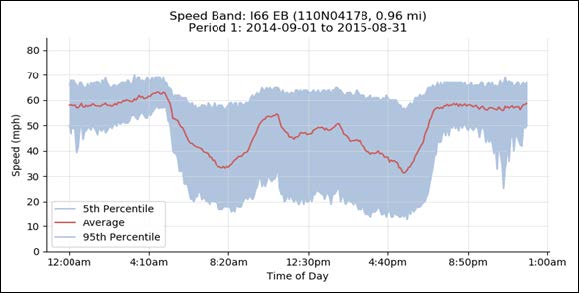
a) Speed band for period 1.
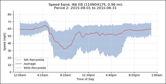
b) Speed band for period 2.
Source: FHWA Probe Data Analysis Tool: Summary of Case Studies
Figure 17. Charts. Compound figure depicts speed band comparison for I-66 eastbound.
Evaluate Breakdown Probabilities
This step in the method requires the use of traffic sensors on the facility of question to gather speed/flow/density data on a lane-by-lane basis. Sensors should ideally be located just upstream of all existing and potential bottlenecks along the stretch of the facility where the shoulder will be opened to traffic. Generally, this will be immediately upstream of on-ramp merges. If the detectors are placed in (or just downstream of) the actual bottleneck, which is just downstream of the ramp merge, they will rarely, if ever, register speeds below the speed at capacity, nor will they count volumes greater than the capacity of the bottleneck.
If archived data from an existing freeway is available, it can be used to determine the probability that traffic flow will break down (i.e., become congested) in the next time interval based upon speed and volume conditions in the present time interval. Two established techniques for conducting this analysis are the product limit method (PLM) and the maximum likelihood technique, which are both based on the statistics of sensor data. These methods must use volume and speed data collected upstream of a bottleneck to reliably predict congestion. Both methods are described in appendix C.
The probability of a traffic breakdown is a function of the flow rate. It represents the capacity distribution function of the freeway segment under investigation, assuming that capacity is a random variable rather than a constant value. The methods for stochastic capacity analysis are usually applied based on flow data aggregated in small time intervals (e.g., 5 minutes) in order to estimate the probability that traffic will break down in the next time interval. For deriving decision parameters for D-PTSU, however, it is typically necessary to predict the risk of a traffic breakdown about 15 minutes in advance because of the "sweep time" that is required to open the shoulder once a breakdown is expected. "Sweep time" includes the time for an agency to verify the shoulder is free of obstructions (by driving the route or inspecting it with closed-circuit television cameras) and conduct other protocols such as notifying law enforcement. The short-term development of traffic demand can either be predicted by time series analysis or be considered within the methods for traffic breakdown analysis by incorporating a time offset. In this case, the occurrence of a traffic breakdown is related to the volume measures (about) 15 minutes prior to breakdown rather than the volume immediately before breakdown.
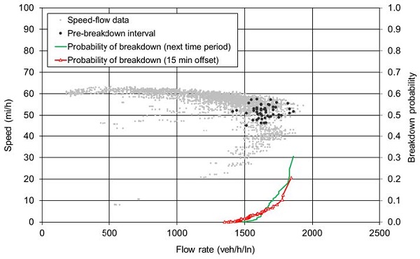
Figure 18 shows analysis results using one the statistical techniques noted above—PLM—for the morning and afternoon peak period using a year of weekday data collected on a freeway in California. Data was downloaded from the California Department of Transportation's Performance Measurement System (PeMS) and initially collected from permanent sensors on the roadway. As traffic breakdowns at low volumes are often caused by crashes or incidents, which cannot be predicted and therefore shouldn't be part of a breakdown prediction model, only intervals at flow rates of more than 1,000 vehicles per hour per lane (veh/h/ln) were considered for estimating the breakdown probability. The estimation was carried out with and without a time offset of 15 minutes (three 5-minute intervals).
a) Morning peak (6 – 10 a.m.).
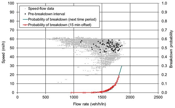
b) Afternoon peak (Noon – 6 p.m.).
Source: FHWA
Figure 18. Charts. Compound figure depicts sample Product Limit Method analysis for the morning and afternoon peak on a freeway in California.
In figure 18, the individual data points indicate speed and flow conditions from a 5-minute time period, with the black points indicating time periods just prior to breakdown. The two curves indicate the probably, for a given flow rate, that traffic flow will break down in the next 5-minute interval (green line with no symbols) or 15 minutes in the future (red line with triangle symbols). The lines stop where flow rates are approximately 1,800 veh/hr/ln and the resulting probably is 20–30 percent. In other words, because freeway capacity is not a constant value, there is no flow rate where breakdown always follows (in either next 5 minutes or 15 minutes into the future). The presence of gray data points (not followed by breakdown) at the same flow rate as black data points (followed by breakdown) is an illustration of this.
The results in figure 18 reveal a higher variance of the breakdown probability distributions with 15-minute time offset compared with the distribution without time offset. This can be explained by the uncertainty of the demand development during the time offset, which influences the variation of the breakdown prediction. However, the differences between the curves are small, particularly at low breakdown probabilities.
The distributions given in figure 18 represent the probability of a traffic breakdown following a single 5-minute interval with a certain traffic volume. During a period of several succeeding intervals at similar volumes, each incorporating the risk of a traffic breakdown, a higher total probability that traffic breaks down during that period arises. Therefore, and because of the stochastic variability of traffic breakdown occurrence, it is useful to apply volumes at low 5-minute breakdown probabilities (e.g., in the range of 1–5 percent) as decision parameters for opening the shoulder. In the example, the volumes at 1 percent and 5 percent probability of breakdown roughly amount to 1,500 and 1,650 veh/h/ln, respectively
Explore Breakdown Distributions
The PLM estimation results in a list of breakdown events,2 or specifically a flow rate observation just prior to the breakdown event. Each of these breakdown events represents a data point that can be used to asses when (time of day and day of week) breakdowns occur on the facility.
Figure 19 shows the distribution of breakdown events for the facility introduced above by day of week and time of day. The figure covers a 1-year analysis period of weekdays.
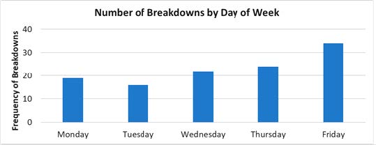
a) Breakdowns by day of week.
b) Breakdowns by hour of day.
Source: FHWA
Figure 19. Charts. Compound figure depicts temporal distribution of breakdown events.
The following observations can be made from figure 18:
- Breakdowns occur slightly more often on Fridays.
- Breakdowns are not a daily event with only 16 (Tuesdays) to 34 (Fridays) days out of 52 weeks experiencing a breakdown event.
- The majority (90 percent) of breakdowns occur between 1 p.m. and 7 p.m.
- More than half (55 percent) of breakdowns occur between 3 p.m. and 6 p.m.
- Breakdowns occur occasionally during midday periods and in the evenings after 9 p.m.
Using these data to assess the viability of a PTSU system leads to the conclusion that a dynamic system may be viable. Specifically, a 3-hour S-PTSU system, active from 3 p.m. to 6 p.m. would miss 45 percent of breakdown events in the figure 18 example. At the same time, a 6-hour S-PTSU system active from 1 p.m. to 6 p.m. would result in many unnecessary openings. For example, from a total sample of 250 working days, only 9 breakdowns are observed to occur in the 1-2 p.m. hour and 14 occur during the 2–3 p.m. hour. Given the temporal variability and the fact that not all weekdays result in a breakdown, a D-PTSU system appears a reasonable option for this facility.
Estimate Initial Decision Parameter Threshold
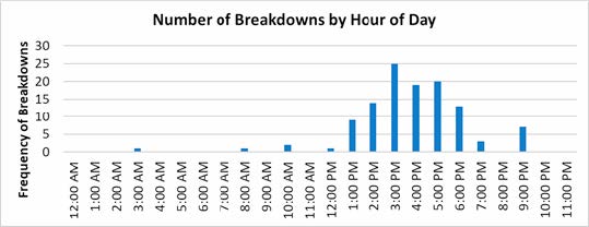
Using the collected speed-flow data, the agency can develop an initial understanding of potential speed-based or volume-based decision parameters for the subject facility. The HCM can provide generalized findings from default speed-flow curves for basic freeway sections to select some initial starting values for opening the shoulder or assessing the feasibility and benefits of PTSU on a specific freeway or throughout a specific region (see example in figure 20).
Source: Highway Capacity Manual, Sixth Edition. 2016. Exhibit 12-7, Speed Flow Curve for Basic Freeway Section, Transportation Research Board, Washington, DC.
Figure 20. Chart. Using Highway Capacity Manual speed-flow curves to select thresholds.
In this example, after consulting the HCM speed-flow curves, the agency has selected 1,500 pc/h/ln as its shoulder opening volume threshold, and 50 mi/h as its shoulder opening speed threshold. The 50-mi/h threshold ensures that congestion will decision parameter consideration of opening the shoulder lane. The passenger cars threshold is set significantly below capacity so that the agency operator will have adequate advance notice to ensure that the shoulder is clear before opening the shoulder. As the operator gains experience, this volume threshold may be adjusted.
Note that the HCM passenger car threshold needs to be converted to the equivalent measure of veh/h/ln so that the operator can readily spot when volumes counted by a sensor exceed the threshold. The passenger car threshold is translated into equivalent vehicles per hour based on the HCM heavy vehicle adjustment factor (which varies with percentage heavy vehicles, terrain, and grade) and the peak hour factor for the facility. In the HCM, see equation 12–9, chapter 12, Basic Freeway Segments for the appropriate values.
Selection of Speed Threshold for Congestion. The HCM speed-flow diagram for basic freeway sections (see figure 20) suggests that a speed threshold of 50 mi/h would be appropriate for determining when a freeway is congested. In reality, breakdown speeds from facility to facility can vary from approximately 40 to 55 mi/h.
Figure 21 shows an example speed-flow plot that includes a year's worth of 5-minute data for the weekday morning peak period for a freeway in Northern California (approximately 16,000 data points). From this example it appears that speeds above 55 mi/h typically indicate uncongested operations on the freeway. Speeds below 40 mi/h typically indicate congested operations. Speeds in between 40 and 55 mi/h may or may not indicate congested (breakdown) operations.
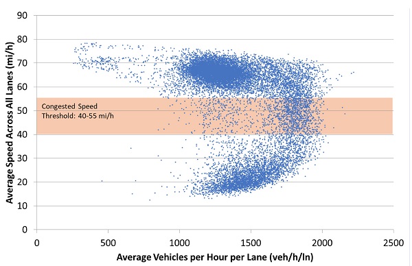
Original figure © Richard Dowling, Alexander Skabardonis, David Reinke. 2008. "Predicting the Impacts of ITS on Freeway Queue Discharge Flow Variability." Transportation Research Record 2047. (See acknowledgments)
Figure 21. Chart. Identification of threshold for congested speeds.
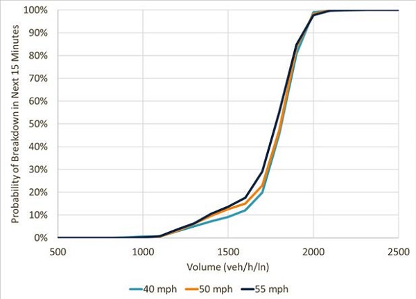
Figure 22 shows the results of a more detailed examination of the data. For each sequence of four 5-minute periods, the first period was examined to determine if the speed was above the selected speed threshold, and if one of the following 5-minute periods fell below the same threshold. If so, the volume of the first 5-minute period was considered to be a pre-breakdown flow rate. All of the pre-breakdown flow rates were then grouped into 100 veh/h/ln bins in a spreadsheet to obtain a probability distribution for the pre-breakdown flow rate. This examination was repeated for three possible congested speed thresholds (40, 50, 55 mi/h). The results are plotted in figure 22. As can be seen in the figure, the distributions are relatively similar, regardless of the selected congested speed threshold. So, in this case the HCM speed threshold for congestion of 50 mi/h is appropriate for this facility and will be used in the remainder of this illustrative example.
Source: FHWA
Figure 22. Chart. Probability of breakdown in next 15 minutes.
Selection of Volume Threshold for Opening Shoulder. The agency operator has two objectives for the selected volume threshold for opening the shoulder to traffic.
- The threshold should be high enough so that the agency is not opening the shoulder when congestion is not imminent.
- The threshold should be low enough so that the agency has adequate time to conduct a sweep and complete the opening process before the onset of congestion.
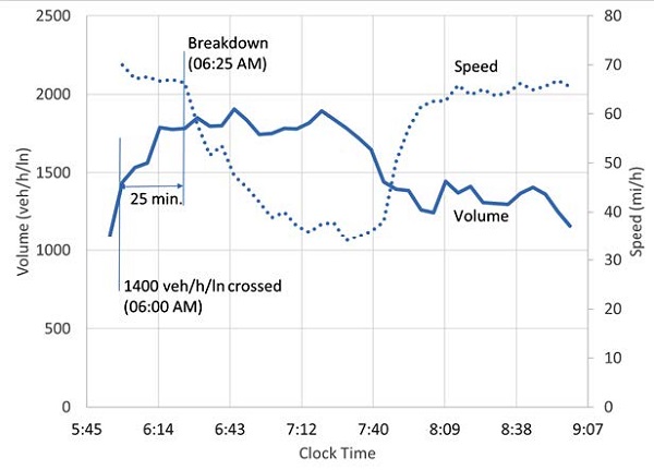
Examination of the cumulative probability curves in figure 22 suggests that at 1,750 veh/h/ln there is a 50 percent probability of breakdown in the next 15 minutes. However, at this threshold, will the agency have enough time to verify the shoulder is clear and open it before congestion is reached? To answer this question the volume and speed trends are examined for several representative days (see figure 22 for one example). From this examination it is determined that if the agency were to use a 1,750 veh/h/ln threshold, it would often have less than 5- or 10-minutes' warning before the onset of congestion. However, if the agency selects a volume threshold of 1,400 veh/hr/ln, it would often have 20 to 25-minutes warning of impending congestion. The amount of time needed to open the shoulder will vary from facility to facility, but most U.S. D-PTSU facilities take more than 5 or 10 minutes.
Source: FHWA
Figure 23. Chart. Example a.m. peak period speed-flow data for one day.
Use of Occupancy. Occupancy is defined by the HCM as 1) the proportion of roadway length covered by vehicles or 2) the proportion of time a roadway cross section is occupied by vehicles. Agencies with PTSU facilities interviewed as part of this project did not report the use of occupancy as a decision parameter, but it could be used as such. Unlike speed values, occupancy values change incrementally in lower-volume conditions and potentially provide an earlier indication of an approaching breakdown. Occupancy values are also less sensitive to fluctuations in capacity. For these reasons, may also wish to consider occupancy-based decision parameters.
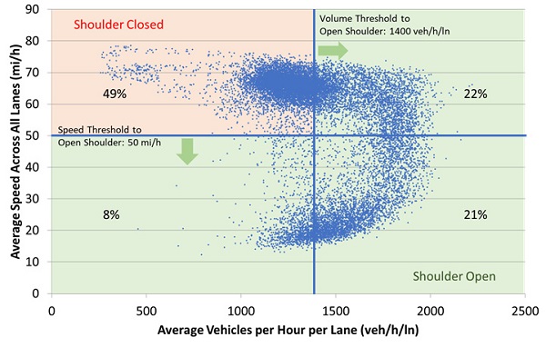
Examination of Full Year Operations. Once the speed and volume thresholds for opening the shoulder have been selected, the agency might plot those thresholds against the speed-flow data to get an understanding of what percentage of the year the shoulder will be open to traffic. Figure 24 illustrates such a plot for a 50 mi/h speed threshold and a 1,400 veh/h/ln volume threshold. In this particular example, the shoulder would be closed for 49 percent and open for 51 percent of the time during the weekday morning peak periods over the course of a year.
Original figure © Richard Dowling, Alexander Skabardonis, David Reinke. 2008. "Predicting the Impacts of ITS on Freeway Queue Discharge Flow Variability." Transportation Research Record 2047. (See acknowledgements)
Figure 24. Chart. Annual percent of time shoulder is open or closed in a.m. peak.
Method III: Macroscopic Decision Parameter Optimization
The HCM 6th Edition freeway facilities methodology allows for analysis of access-controlled freeway and highway facilities in under-saturated and congested conditions over multiple analysis periods (up to 24 hours at a time). The methodology provides macroscopic operational analysis that combines the HCM's basic freeway, merge/diverge, and weave segment methodologies, and further extends them to model queue spillback and queue dissipation across adjacent segments. The methodology has extensions for both reliability and active transportation and demand management strategies. Most importantly for this document, it includes guidance for modeling shoulder-use strategies that increase overall facility capacity in the PTSU segments.
With the goal of determining the relative effectiveness of multiple decision parameter types under varying demand scenarios, the freeway facilities methodology provides a useful framework on which to develop, test, and compare sets of strategies. In comparison to more detailed analysis approaches like microsimulation, the method provides a more efficient analysis approach for analyzing hundreds or even thousands of scenarios. FREEVAL, which was developed as a part of the HCM 6th Edition update, is a free open-source implementation of the freeway facilities methodology. Several modifications to FREEVAL were made to conduct the research described in this chapter and enable more responsiveness to traffic conditions and more realistic durations for changing the number of lanes on the freeway (i.e., opening or closing the shoulder) and these are described in appendix C. FREEVAL and the HCM freeway facility were the basis for developing the guidance for D-PTSU decision parameter implementation described below.
In this report, the application of the FREEVAL methodology is introduced using a generic example facility with illustrative volume profiles. The results presented below provide useful insights in the tradeoffs of different decision parameters as a function of congestion levels (d/c ratios) and demand patterns (slope of demand curve). But in addition to these generic results, a facility-specific application of the method could be used to explore these tradeoffs and benefits of different D-PTSU decision parameters for a specific facility.
Experiment Design
The FREEVAL experiment was designed to test two different types of PTSU decision parameters: speed-based and volume-based. Operational performance of the facility was then determined for each decision parameter under multiple demand scenarios. Both the peak bottleneck demand as well as the rate (slope) of the demand increase were varied. In order to maintain consistency across geometries with differing numbers of lanes, peak bottleneck demand volume was considered in relation to the bottleneck capacity, and thus represented as the d/c ratio. In the results presented in this chapter, capacity values represent the capacity of the general purpose lanes only and not the shoulder. Thus, PTSU facilities are able to process d/c ratios greater than 1.0 when the shoulder is open.
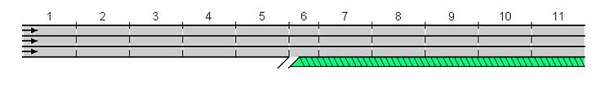
Three different geometric configurations for the facility, shown in figure 25, were considered in the experiment. The configurations differed either in the cause of the bottleneck (i.e., merge vs diverge) or the configuration of the shoulder use facility (i.e., beginning at an on-ramp or flowing through an on-ramp). Each geometry was also considered for two-lane, three-lane, and four-lane (per direction) facilities. The three configurations for facilities with three mainline lanes per direction are shown below, with a crosshatched green area showing a shoulder used as a part-time lane. The terminology "Type A" and "Type B" was created for purposes of this report.
a) Merge bottleneck with PTSU beginning at the ramp (Type A).
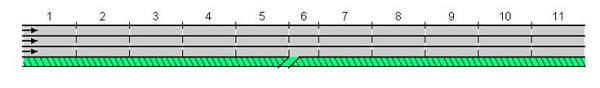
b) Merge bottleneck with PTSU extending through the ramp (Type B).
c) Diverge Bottleneck with PTSU extending through the ramp.
Source: FHWA
Figure 25. Diagrams. Compound figure illustrates ramp-freeway junction types in FREEVAL experiment.
All three facilities were subject to the following fixed assumptions:
- Full lane capacity, non-bottleneck (2,400 pc/lane/hour).
- Full lane capacity, bottleneck (2,100 pc/lane/hour).
- Free-flow speed (70 mi/h).
- Facility sweep time (20 minutes).
- Facility clearance time (20 minutes).
- Minimum duration shoulder must remain open (15 minutes).
- Heavy vehicle percentage (1 percent single-unit trucks, 1 percent tractor trailers).
- Length of time bottleneck is at peak demand (30 minutes).
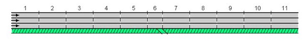
The operational status of a corridor in the time frame leading up to a breakdown can vary significantly for different facilities. One primary cause of this is the rate at which the demand volumes increase from below capacity to above capacity. This is referred to as "slope offset" in this chapter. Some facilities experience rapid increases in demand, while others may see volumes increase more gradually. For example, demand tends to increase more rapidly in the morning peak than in the afternoon peak or on weekends. For the purpose of this experiment, this variation is modeled through different slope offsets for the demand profiles. Specifically, this experiment considered six different slopes. Figure 26 shows the demand profiles for a three-lane facility with a target peak d/c of 1.1 and a 90-percent volume decision parameter threshold.
Source: FHWA
Figure 26. Chart. Demand profiles for three-lane facility.
The profiles represent an increase of demand volumes from a d/c ratio well below 1.0 up to the max bottleneck d/c defined as an exponential function (V = V0*et). Differing exponential slopes were created by offsetting (delaying) the start of the demand increase by increments of 10 minutes for a range of no offset (zero) up to 50 minutes. A slope offset of zero means the demand begins to increase immediately, but at a very gradual rate. A higher slope offset delays the starting point of demand increases, resulting in a steeper demand profile. A low slope offset (flatter slope) provides more time between a decision parameter volume being reached and the demand profile exceeding capacity, than a higher slope offset (steeper slope).The above chart shows an example of the six demand profiles for a three-lane facility with a peak bottleneck d/c of 1.0. For reference, a line showing where a 90 percent volume decision parameter threshold is met is also shown.
The slope of the demand curve was one of the six key parameters that was varied in the experiment: (1) the geometric configuration of the bottleneck as described above), (2) the number of main line lanes, (3) the capacity of the shoulder, (4) the peak bottleneck d/c ratio, (5) the demand profile slope described above, and (6) the decision parameter threshold itself. Table 9 summarizes the parameter variations of the experiments and a total resulting 5,670 scenarios analyzed.
| Parameter | # | Values |
|---|---|---|
| Geometric bottleneck configuration | 3 | Type A Merge, Type B Merge, Diverge |
| Number of mainline lanes | 3 | 2, 3 and 4 lanes |
| Shoulder capacity | 3 | 1,200 pc/h/ln, 1,400 pc/h/ln, 1,600 pc/h/ln |
| Peak bottleneck demand-to-capacity ratio | 5 | 1.02, 1.04, 1.06, 1.08, 1.10 |
| Demand volume profile shape/slope | 6 | 0 to 50-minute offsets |
| Decision parameter threshold | 7 | See below |
| Total Scenarios | 5,670 | 3*3*3*5*6*7 |
pc/h/ln = passenger cars per hour per lane.
For the decision parameter threshold, both volume- and speed-based decision parameters were evaluated. In the case of a speed-based decision parameter, the shoulder was opened when observed speeds dropped below the specified value. For a volume-based decision parameter, the shoulder was opened when volumes were first observed above the specified value (given as a percentage of a bottleneck's known capacity). Table 10 shows the different thresholds considered for the two decision parameter types.
| Decision Parameter Type | # | Threshold |
|---|---|---|
| Speed | 3 | 45 mi/h, 50 mi/h, 55 mi/h |
| Volume (as a percentage of bottleneck capacity) | 4 | 70%, 80%, 90%, 100% |
Results
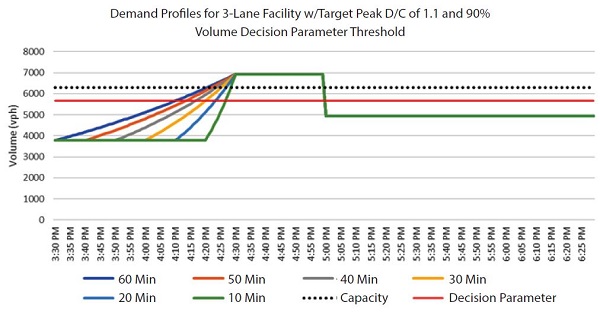
The rate of the volume increase leading up to the breakdown is crucial when identifying a decision parameter. Historical data of typical volume rate increases can be used to inform when how realtime conditions will change the coming minutes and whether shoulder-opening activities should be initiated or not.
Once the necessary software modifications were made to enable the execution of the experiment in the FREEVAL computational engine, all scenarios were run and a set of performance metrics were recorded. While the core HCM methodology provides a variety of performance metrics, the primary metric for this analysis is the delay experienced on the facility during the study period, which is recorded as the vehicle hours delay (VHD). Beyond delay, an additional key performance metric specific to this experiment is the number of analysis periods that the shoulder was opened for each scenario.
The primary result of the HCM experiment shows that the rate of the volume increase leading up to the breakdown is crucial. While varying parameters such as number of mainline lanes, peak d/c ratio, and shoulder capacity changed the magnitude of the values, the conclusions reached across the variations were all largely consistent. For instance, while higher peak bottleneck d/c ratios influenced the overall extent of delay experienced, the relative effects of the different shoulder-use decision parameters were essentially fixed across all five values. As a result, no matter how advanced realtime data collection on a facility may be, historical data provides valuable insight into whether an observed volume increase is expected to be sustained or not. Figure 27 illustrates this relationship.
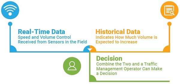
Source: FHWA
Figure 27. Chart. Use of realtime and historical data for part-time shoulder use decisionmaking.
Figure 28 demonstrates this for a three-lane Type A merge facility with a medium rate of demand increase (offset = 30 minutes). While the VHD values shown in the top half of the figure do vary across d/c ratios ranging from 1.02 up to 1.10, the relative delay experienced by each decision parameter scenario is similar for all cases. This is further reflected by examining the number of periods the shoulder is open in each case, which are almost identical across all five d/c values. This same trend is found for nearly all variations of facility geometry.
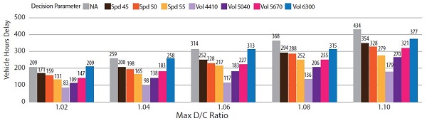
a) Vehicle hours of delay by decision parameter and max d/c.
b) Periods shoulder is open by decision parameter and max d/c.
Source: FHWA
Figure 28. Chart. Effects of varying peak bottleneck d/c ratios for a three-lane, Type A facility geometry and demand increase slope (offset = 30, medium).
The top chart shows vehicle hours of delay when different speed thresholds (gray/orange/tan bars) and volume thresholds (purple bars) determine when the shoulder is opened. Each group of bars represents a different d/c ratio, and volumes and geometry are consistent across all scenarios. The bottom chart shows the number of minutes in the hour the shoulder is open. In general, higher speed and lower volume thresholds result in the shoulder being opened longer and delay being lower. This represents a tradeoff for agencies to consider.
Generalized Results
As previously discussed, the capacity of freeway bottlenecks varies greatly, and the thresholds at which the PTSU opening process should begin to avoid the onset of a breakdown will vary. However, making a number of assumptions, tables indicating the minutes until breakdown occurs for various scenarios can be developed. A set of tables developed for this project can be found in appendix D, and one example is shown below in table 11.
| Bottleneck Per Lane Capacity | Minutes until Capacity Is Reached | |||||||||
|---|---|---|---|---|---|---|---|---|---|---|
| Increase in Hourly Volume Rate In Past 5 Minutes | ||||||||||
| 1,900 | 10 | 20 | 30 | 40 | 50 | 60 | 70 | 80 | 90 | 100 |
| Current Volume (veh/h/ln) | ||||||||||
| 0 | 190 | 95 | 64 | 48 | 38 | 32 | *28 | *24 | *22 | *†19 |
| 100 | 180 | 90 | 60 | 45 | 36 | 30 | *26 | *23 | *20 | *†18 |
| 200 | 170 | 85 | 57 | 43 | 34 | *29 | *25 | *22 | *†19 | *†17 |
| 300 | 160 | 80 | 54 | 40 | 32 | *27 | *23 | *20 | *†18 | *†16 |
| 400 | 150 | 75 | 50 | 38 | *30 | *25 | *22 | *†19 | *†17 | *†15 |
| 500 | 140 | 70 | 47 | 35 | *28 | *24 | *20 | *†18 | *†16 | *†14 |
| 600 | 130 | 65 | 44 | 33 | *26 | *22 | *†19 | *†17 | *†15 | *†13 |
| 700 | 120 | 60 | 40 | *30 | *24 | *20 | *†18 | *†15 | *†14 | *†12 |
| 800 | 110 | 55 | 37 | *28 | *22 | *†19 | *†16 | *†14 | *†13 | *†11 |
| 900 | 100 | 50 | 34 | *25 | *20 | *†17 | *†15 | *†13 | *†12 | *†10 |
| 1,000 | 90 | 45 | *30 | *23 | *†18 | *†15 | *†13 | *†12 | *†10 | *†9 |
| 1,100 | 80 | 40 | *27 | *20 | *†16 | *†14 | *†12 | *†10 | *†9 | *†8 |
| 1,200 | 70 | 35 | *24 | *†18 | *†14 | *†12 | *†10 | *†9 | *†8 | *†7 |
| 1,300 | 60 | *30 | *20 | *†15 | *†12 | *†10 | *†9 | *†8 | *†7 | *†6 |
| 1,400 | 50 | *25 | *†17 | *†13 | *†10 | *†9 | *†8 | *†7 | *†6 | *†5 |
| 1,500 | 40 | *20 | *†14 | *†10 | *†8 | *†7 | *†6 | *†5 | *†5 | *†4 |
| 1,600 | 30 | *†15 | *†10 | *†8 | *†6 | *†5 | *†5 | *†4 | *†4 | *†3 |
| 1,700 | * | *†10 | *†7 | *†5 | *†4 | *†4 | *†3 | *†3 | *†3 | *†2 |
| 1,800 | *†10 | *†5 | *†4 | *†3 | *†2 | *†2 | *†2 | *†2 | *†2 | *†1 |
| 1,900 | *†0 | *†0 | *†0 | *†0 | *†0 | *†0 | *†0 | *†0 | *†0 | *†0 |
| 2,000 | -- | -- | -- | -- | -- | -- | -- | -- | -- | -- |
| 2,100 | -- | -- | -- | -- | -- | -- | -- | -- | -- | -- |
| 2,200 | -- | -- | -- | -- | -- | -- | -- | -- | -- | -- |
veh/h/ln = vehicles per hour per lane.
-- = not applicable.
* Operator should consider initiating shoulder-opening activities.
† The freeway will reach capacity before the shoulder is opened.
Suppose a freeway has an hourly volume of 1,200 veh/h/ln, and the capacity of a downstream bottleneck is 1,900 veh/h/ln. Also suppose it takes 20 minutes to "sweep" the shoulder and complete the opening process once the decision to open the shoulder has been made. Find the "1,200'" row on the table. If the hourly volume rate increased 10 veh/h/ln in the last 5 minutes (first column of data in the table) and that rate of increase is assumed to continue, it will be 70 minutes until capacity is reached. Moving further to the right, the minutes until capacity is reached decrease. When they fall below 20 minutes, values are displayed in red to indicate the shoulder cannot be opened before capacity is reached due to the sweep time.
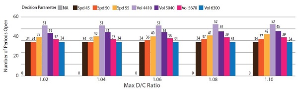
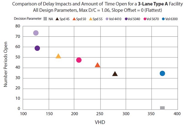
Figure 29 and figure 30 highlight some of the differences in behavior resulting from varying the rate of increase of the demand profile. Both figures compare the VHD with the number of periods the shoulder was opened for a three-lane merge Type A bottleneck with a peak bottleneck d/c ratio of 1.06. Figure 29 plots the metrics for the facility under the slowest rate of demand volume increase (offset = zero). Notice that the chart shows a wide degree of spread across various decision parameter types and thresholds. In contrast, figure 30 shows results for the same facility but under the fastest rate of demand increase (offset = fifty minutes). Unlike in figure 28, the points are all clustered together, with little variation in results regardless of decision parameter type or threshold. Taken together, this indicates that the choice of decision parameter type or threshold is less important for facilities that experience sudden or rapid increases in demand volume. Alternatively, when the volumes increase to an over-capacity condition more slowly, the choice of decision parameter type and threshold plays a much larger role in the overall performance of PTSU.
Source: FHWA
Figure 29. Chart. Comparison of vehicle hours delay and number of periods the shoulder is open for a three-lane Type A merge facility for a peak demand-to-capacity ratio of 1.06 and no slope offset.
Overall, the results from the HCM experiment have two primary findings. First, it is possible to develop general guidance largely based on the rate of increase in demand experienced in the time leading up to capacity being exceeded. Facilities with more gradual rates of change should focus more on decision parameter type and threshold, while those with rapid demand increases will see fewer practical differences between different types of decision parameters. This in turn leads to the second takeaway, which is that if field-observed data for both the ratio of peak demand versus capacity and the rate of increase in demand leading up to breakdown are known, they will likely be very indicative of the performance of PTSU and should be used to inform decisionmaking to determine decision parameter type and threshold.
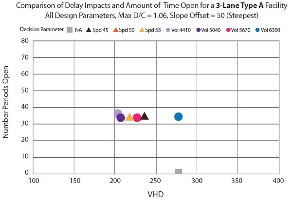
Source: FHWA
Figure 30. Chart. Comparison of vehicle hours delay and number of periods the shoulder is open for a three-lane Type A merge facility for a peak demand-to-capacity ratio of 1.06 and a 50-minute slope offset.
Method IV: Microscopic Decision Parameter Refinement
Microsimulation offers a way to evaluate and refine a D-PTSU decision parameter scheme prior to implementation in the field. While the macroscopic optimization in Method III is geared at efficiently running a large number of potential decision parameter events and combinations, Method IV is designed to test a select few decision parameter strategies in a more dynamic simulation environment.
Microsimulation models individual vehicle movements using a series of behavioral rules or algorithms, including car-following, lane changing, gap acceptance, and others. Microsimulation tools are frequently used to evaluate freeway systems, proposed interchange geometric changes, and active traffic and demand management strategies.
Microsimulation tools can be used to model S-PTSU and D-PTSU systems, with the latter using whatever desired combination of decision parameter events and decision algorithms of interest through the use of Component Object Model (COM) scripting. Using COM, many microsimulation tools can use customized and agency-specific decision algorithms.
In a typical work flow, an agency may employ Methods I and II to understand the congestion and demand patterns on the subject facility, and then use Method III to test a range of potential decision parameter options and combinations. Method IV then applies the developed decision parameter logic to the subject facility in a dynamic simulation context.
Similar to the discussion of Method III, the microscopic decision parameter refinement is best applied to the specific facility on which an agency is considering PTSU. In this section, the method is applied to a generic facility that mirrors the Method III experiment to illustrate the application of the method. The section first discusses experimental design for the microsimulation analysis and then summarizes key simulation findings. The same steps can be applied to both a microsimulation analysis of other geometric configurations as well as decision parameter algorithms.
Experiment Design
The microsimulation experiment was designed to test two different types of D-PTSU decision parameters (i.e., speed-based and volume-based). Operational performance of the facility was then determined for each decision parameter under multiple demand scenarios. This experiment used the VISSIM microsimulation tool, but other tools are viable as long as they can model freeway operations and allow the use of custom logic scripts through COM.
Scenario Demand Variations: The same vehicle demand and rate (slope of the demand increase) discussed for the FREEVAL experiments (figure 25) was used for the simulation scenarios. This was to maintain consistency between the FREEVAL and simulation experiments, which will allow for results comparison.
Decision Parameter Variations: Four decision parameter types were considered. These include two speed decision parameter scenarios (45 mi/h and 55 mi/h) and two volume decision parameter scenarios (70 percent and 80 percent of bottleneck capacity). A base scenario without the D-PTSU (i.e., no decision parameter, no opening of shoulder) was also analyzed to provide baseline comparison. It should be noted that only a select number of decision parameter scenarios were analyzed in microsimulation, compared to the FREEVAL experiments, due to the increased time involved in developing and analyzing simulation models.
Geometric Configuration: Only the merge bottleneck with Type B geometry (i.e., merge bottleneck with PTSU flowing through the ramp, see the discussion on Method III above) was considered in the simulation. A three-lane geometry (not including the shoulder) for the mainline was considered for the facility with PTSU.
Table 12 summarizes the parameter variations of the experiments and resulting total number of scenarios analyzed in the simulation.
| Parameter | # | Values |
|---|---|---|
| Geometric bottleneck and shoulder configuration | 1 | Type B Merge |
| Number of mainline lanes | 1 | 3 lanes |
| Shoulder capacity | 1 | 1,600 vph |
| Decision parameter variations | 5 | No Decision parameter, Speed=45mi/h, Speed=55 mi/h, Vol=0.7*d/c, Vol=0.8*d/c |
| Peak bottleneck d/c ratio | 5 | 1.02, 1.04, 1.06, 1.08, 1.10 |
| Demand volume profile shape/slope | 6 | 0 to 50-minute offsets |
| Total Scenarios | 150 | 1*1*1*5*5*6 |
d/c = demand to capacity (ratio). vph = vehicles per hour.
The following fixed assumptions were made for the simulation experiments:
- Full lane, non-bottleneck capacity was assumed as 2,400 pc/h/ln.
- Full lane, bottleneck capacity was assumed as 2,100 pc/h/ln.
- Shoulder capacity was assumed as 1,600 pc/h/ln.
- A free-flow speed of 65 mi/h was assumed.
- Facility sweep time to open the shoulder was set to 20 minutes.
- Minimum duration for the shoulder to stay open was set to 15 minutes.
- A 2 percent heavy vehicle presence was considered.
It should be noted that capacity in simulation is not a value that can be pre-defined by the user. Therefore, the research team conducted sensitivity testing of the car-following behavior parameters (VISSIM's Wiedemann 99) to reasonably represent the capacities of freeway mainline, freeway bottleneck, and shoulder lane. The team then extracted capacities from the model by developing flow-density curves by varying vehicle demand to create various flow regimes.
Realtime Microscopic Analysis
Once a PTSU facility is operational, microsimulation can be used in realtime to inform and optimize PTSU decisionmaking by facility operators. Once a microsimulation model is constructed and calibrated, it can be fed data from field sensors and traffic variables such as speeds, volumes, and vehicle mixes can be updated in real time. This "sensor in the loop" approach enables data to be analyzed, rather than merely observed, by TMC staff, and it enables microsimulation to be linked to realtime, rather than historical, traffic conditions. With this data, microsimulation can be used as a predictor of traffic conditions in the near term (1 hour or less). This would effectively replace a lookup table such as the example in table 11. Integrated corridor management (ICM) is an emerging active traffic management strategy which often implements changes across multiple modes and routes. Pilot ICM installations in Dallas and San Diego have incorporated realtime data into microsimulation in this manner.
VISSIM Results and Conclusions
The following measures of effectiveness were used in VISSIM to summarize results:
- Total network delay.
- Network delay reduction as a function of shoulder duration open.
- Vehicle throughput, both for the mainline and the shoulder.
Figure 31 illustrates network delay comparison under various decision parameters and maximum d/c ratios for slope offset 0 and slope offset 40. As previously described, slope offset represents the number of minutes between the start of the experiment and the start of volume increase. In both experiments, the same peak volume was reached at the same time, so higher slope offset values represent a more rapid rate of volume increase. While results from only two slopes are shown here, simulation results for other slopes indicated similar findings.
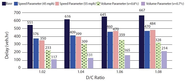
a) Network Delay: Slope Offset = 0; Shoulder Capacity = 1,600 veh/hr.
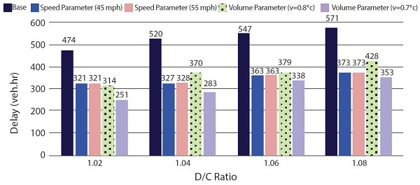
b) Network Delay: Slope Offset = 40; Shoulder Capacity = 1,600 veh/hr.
Source: FHWA
Figure 31. Charts. Compound figure depicts network delay comparison under various decision parameter variations and maximum demand to capacity ratios.
Key network delay findings include:
- For lower slope offset demand variations (e.g., slope = 0, indicating a more gradual volume increase to oversaturation), the volume-based decision parameter outperforms the speed decision parameter and results in considerably lower network delay. In addition, setting up a lower volume decision parameter threshold further reduces network delay by opening the shoulder early before the bottleneck conditions start.
- For the higher slope offset demand variations (e.g., slope = 40, indicating a more abrupt volume increase from below capacity to above capacity), a speed-based decision parameter tends to perform the same and even better in certain conditions.
Figure 32 shows network delay reduction and shoulder open duration under various decision parameter variations and slope offsets for max d/c = 1.02.
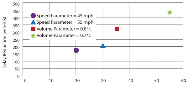
a) Maximum demand to capacity ratio = 1.02; Slope Offset = 0.
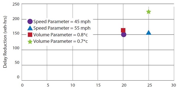
b) Maximum demand to capacity ratio = 1.02; Slope Offset = 40.
Source: FHWA
Figure 32. Charts. Compound figure compares delay reduction and shoulder open duration under various decision parameter variations for different maximum demand to capacity ratios and slope offsets.
Key findings include:
- With the lower slopes (e.g., slope = 0), similar to the network delay findings, the volume-based decision parameter outperforms the speed-based decision parameter by reacting to the volume increase faster and opening up shoulder before the bottleneck conditions are realized. This can particularly be observed from the volume decision parameter = 0.8*d/c scenario, as the shoulder was open for only 5 minutes longer than the speed decision parameter = 55 mi/h scenario (35 minutes vs. 30 minutes), yet substantial delay reductions are achieved.
- With the higher slopes (e.g., slope = 40), the speed-based decision parameter tends to perform similarly to the volume-based decision parameter scenario. For example, the speed decision parameter = 45 mi/h scenario is almost identical to the volume decision parameter = 0.8*d/c scenario. While the findings are counter-intuitive, this can be attributed to the specific demand scenarios that were designed and tested in the experiments. With the abrupt volume jump prior to the breakdown under the high slopes, the volume decision parameter scenarios are unable to respond before the traffic flow breakdowns happen, resulting in performance similar to the speed-based decision parameter scenarios.
Figure 33 illustrates vehicle throughput under slope offset = 0 and maximum d/c ratio = 1.04 under the speed decision parameter = 45 mi/h and the volume decision parameter = 0.8*d/c scenarios. The below figures provides an example of how the volume decision parameter responds quicker to the pre-breakdown conditions by opening the shoulder sufficiently prior to the breakdown and providing additional capacity for a longer period. This can also be observed from the speed decision parameter results as the obtained shoulder throughput was close to capacity (1,600 vehicles per hour) during almost every interval that the shoulder was open, indicating oversaturated conditions had already been reached by the time the shoulder was opened. Finally, throughput results for the speed decision parameter scenario validate the shoulder capacity assumption of 1,600 vehicles per hour used in the simulation.
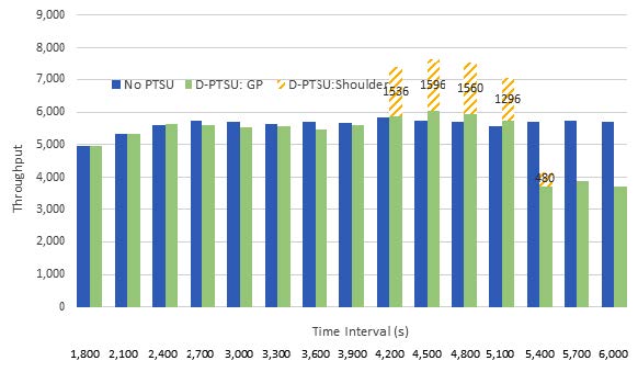
D-PTSU = dynamic part-time shoulder use. GP = general purpose (lanes). PTSU = part-time shoulder use.
a) Vehicle throughput where slope offset = 0, maximum demand to capacity ratio = 1.04, the speed decision parameter = 45 mi/h, and shoulder capacity = 1,600 veh/hr.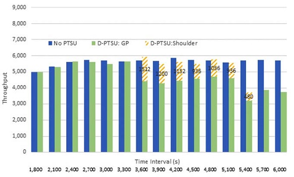
D-PTSU = dynamic part-time shoulder use. GP = general purpose (lanes). PTSU = part-time shoulder use.
b) Throughput: Slope Offset = 0; Max d/c = 1.04; Volume Decision parameter = 0.8*d/c; Shoulder Capacity = 1,600 veh/hr.Source: FHWA
Figure 33. Charts. Compound figure depicts vehicle throughput for slope offset = 0, maximum d/c = 1.04 under speed decision parameter = 55 mi/h and volume decision parameter = 0.8*d/c scenarios.
Method V: Monitoring and Adjustment
The fifth and final method acknowledges the value of continuously monitoring a D-PTSU system once it is in operation. Facility operators learn their facility from observing day-to-day operations and develop an understanding for when to open and close based on the incoming data they are seeing. Whether the system being monitored is a Level 2, 3, or 4 D-PTSU, there is value in monitoring the operations and adjusting thresholds based on experience. The concepts and data analysis methods described in this chapter can reasonably be applied to existing D-PTSU systems to assist with the assessment of ongoing operations.
Conclusions
This chapter presented a method for evaluating the viability of a D-PTSU system for a given facility and provided guidance for exploring and comparing different options for using decision parameters to open the system. In the decision to select an appropriate decision parameter for a D-PTSU facility, three primary choices are available:
- Fixed time-of-day parameters, which pre-determine the hours of operations.
- Volume-based decision parameters, which are proactive and geared toward preventing breakdown from happening in the first place.
- Speed-based decision parameters, which are reactive to breakdown having occurred.
It is recommended that both a speed and a volume threshold be selected for opening the shoulder lane.
The analysis suggests that it is most effective to select both a volume threshold and a speed threshold for opening the shoulder to traffic. This ensures that the low-volume, low-speed conditions typical of congested operations will result in the shoulder being opened, even if the volume threshold may not have been reached. Inclement weather and other conditions can cause speeds to drop below the speed threshold even though volume thresholds have not been reached, reducing the capacity of the facility below its normal, fair weather condition. This situation can also occur when there is a downstream incident backing up traffic into the section with PTSU; however, the agency operator will also want to consider whether there is any value to opening the shoulder when the bottleneck is downstream of the PTSU section. Additionally, an operator can use its discretion and not open the shoulder if they determine weather or other realtime conditions make it unsafe to open the shoulder.
Using sensor technology, speed-based decision parameters are easier to implement, since they are directly tied to a bottleneck sensor. If sensor speed shows decision parameter speed, the shoulder is opened. This requires the use of realtime sensor data, which is best achieved using sensor technology deployed in the field. While probe-based speed data are available to many agencies, they are limited in application for two primary reasons: (a) they are generally not available in realtime, and (b) they are aggregate speeds from a sample of vehicles over a distance rather than speeds measured instantaneously at a point.
Due to the nature of the speed-flow-density relationship, a speed-based decision parameter will typically occur "too late" to prevent breakdown. As was discussed in Methods I and II, a decision parameter speed of 45 mi/h, for example, corresponds to a 100 percent probability of breakdown. However, the macroscopic decision parameter optimization experiment described in this section found that in some cases, a speed-based decision parameter is still the best option as it balances delay impact with the "wasted" time during which the shoulder is open, which can lead to safety concerns.
Volume-based decision parameters are more difficult to implement, since the decision parameter volume is a function of the bottleneck capacity. However, they are better at predicting future traffic conditions. The volume-based decision parameter should be set at a flow rate at which the breakdown probability is still very low, with that breakdown probability obtained from the PLM or maximum likelihood method presented in Method II.
Because a shoulder cannot be opened instantaneously, the rate of volume increase in the minutes beyond the present time is key. Historical data and knowledge of a specific facility can provide into this issue.
Since bottleneck capacity is not fixed but rather depends on site-specific attributes (geometry, vehicle mix, weaving, etc.), it is recommended that a site-specific assessment of breakdown probability be performed. In the Method II example, 95 percent breakdown occurs at a flow rate of 1,570 vehicles per hour per lane. As a result, the decision parameter volume needs to be set at some percentage of that breakdown capacity.
In selecting a volume-based decision parameters, the slope of the demand curve, which describes the rate-of-increase in traffic volume leading up to breakdown, is another key consideration. Given the same decision parameter volume, a flatter slope provides more time between a decision parameter volume and breakdown flow rate, relative to a steeper slope.
The volume-based decision parameter also needs to take into account the amount of sweep time needed between reaching the volume threshold for activating PTSU and the time the shoulder can actually be opened. Specifically, the decision parameter volume needs to be set such that it provides sufficient time between reaching the decision threshold and the breakdown occurring, which is a function of facility length (longer facilities take longer to sweep), sweep technology (camera tour is faster than manually driving it), rate of change of traffic growth (steeper slopes give less time than flatter slopes), and, ultimately, the bottleneck capacity.
At the same time, agencies need to be careful not to set decision parameter volumes too low for two primary reasons:
- Opening the shoulder too early results in increases in capacity before it is needed, resulting in potentially higher speeds, and potentially reduced safety.
- A decision parameter volume that is set too low can result in false positives; i.e., traffic volumes are increasing but will never reach capacity.
Based on the macroscopic experiment, it is recommended that an "optimum" volume threshold for the decision to initiate PTSU be set at about 70–80 percent of breakdown flow rate.
Occupancy could also be used as a decision parameter in addition to or in place of speed and/or volume. Agencies interviewed for this project did not report the use of occupancy-based decision parameters, but it could provide an indication of forthcoming breakdown.
In summary, the three primary decision parameter types—fixed time-of-day, speed-based, and volume-based—are most applicable under the following conditions:
- If breakdowns are frequent and predictable (e.g., every morning between 7 a.m. and 9 a.m., but rare during other times of the day), a fixed time-of-day decision parameter may be sufficient. If there are no breakdowns outside of the peak, there are few benefits to be gained from a dynamic system, and consequently there may be limited value in investing further resources in dynamic decision parameter technology.
- Volume-based decision parameters are most reliable for realtime prediction of oncoming breakdowns. Volume increases as the onset of breakdown approaches, and this incremental change often enables an analyst to predict the breakdown soon enough to initiate a sweep and open the shoulder prior to reaching breakdown conditions. Volume-based decision parameters are most straightforward to apply on freeways with frequent and reasonably predictable congestion patterns, where the rate of volume increase, the driver population, the heavy vehicle percentage, and other parameters of the traffic stream are similar day to day (e.g., breakdown every morning peak).
- Speed-based decision parameters are less reliable indicators of oncoming breakdowns. In general, speed does not substantially decrease until just prior to the onset of breakdown, and there may be insufficient time to conduct a sweep prior to breakdown if a speed-based decision parameter is used. However, volume-based decision parameters should be supplemented by speed-based decision parameters. If a volume-based decision parameter fails to detect the onset of breakdown but speeds begin to decrease, then it may still be appropriate to begin a sweep and open the shoulder. The capacity gained through D-PTSU often relieves the congestion quickly and enables the freeway to "recover" from short-term breakdown. Volume-based decision parameters are most likely to "miss" an oncoming breakdown—and a supplemental speed-based decision parameter is likely to be activated—on freeways where breakdown is a not a routine, predictable occurrence.
To account for both breakdown types, those originating from daily demand patterns and those originating from random fluctuation, it is useful to have both decision parameter types included in a D-PTSU system. Having both a volume-based and a speed-based decision parameter will also provide operators with the most flexibility in adjusting decision parameter thresholds during the ongoing monitoring of a D-PTSU system.
1PTSU was entirely removed from I-66 in 2018 as part of a major widening project. [ Return to note 1. ]
2The Highway Capacity Manual defines a breakdown as "the transition from noncongested conditions to congested conditions typically observed as a speed drop accompanied by queue formation." (See TRB 2016) [ Return to note 2. ]