Scoping and Conducting Data-Driven 21st Century Transportation System AnalysesModule 1. Characterizing System Dynamics and Diagnosing ProblemsModule 1 characterizes the performance of the transportation system and identifies and diagnoses system problems (see Figure 4 on the following page). Is the system performing as expected? Is travel in the system safe, reliable, and predictable? Module 1 also considers the role of analytical projects: What types of analytical projects can be successfully conducted in support of improving system performance? Analysts are often not directly involved in this part of the system management process. In many cases, the analyst becomes involved after an analytic project concept has been developed. More precisely, an analyst may be asked only to respond to an assignment to conduct a specific analytic project. Too often, they are not engaged in characterizing the performance of the system or offering insights on the problems within the system. This is unfortunate, since analysts work directly with the data and tools that provide insight into the underlying nature and dynamics of the transportation system. If an analyst has just completed a reliability analysis of trips within the system and potential mitigation strategies, the insight gained from this analysis may be critical for understanding the complex interaction of factors driving delays and outlier travel times in the system. System users may experience a lack of travel-time reliability, and system manager may observe that the system has "bad days". However, the analyst who has systematically assessed the root causes of unreliability, can point to specific conditions (low visibility, spotty slick conditions, incidents in particular hot spots, and shifted travel demand based on delayed area-wide school start times) and the resulting impact on travel-time variability. Any discussion of improving system reliability occurs at a deeper, more informed, more data-driven level. To implement the 21st Century Analytic Project Scoping Process as a continuous process, key inputs for characterizing the system dynamics include the data used in related (previous and current) analyses, the hypotheses and findings of these studies, and the insights gained by the analysts who conducted these studies. As illustrated in Figure 4, this module describes a step-by-step process that engages the 21st Century analyst and brings analytical capital to bear to enhance and improve subsequent analyses, system management, and system performance. First, we discuss the nature of system performance measures that reflect system products and by-products—and how to reconcile differing stakeholder viewpoints of what "good" performance looks like. Second, we discuss how time-variant profiles of key measures can be useful in bringing depth and clarity to deliberations on system performance and how early diagnostic activities can guide the development of preliminary analytic problem statements. Third, these concise statements of underlying need and analytic intent are a critical building block used to intelligently integrate, characterize, and prioritize analytical projects prior to larger-scale scoping and execution. It is here, in the earliest origins of individual analytical projects, that poor decisions are often made that greatly reduce the value of downstream analytical activity. Effective planning for analytics is a project portfolio management effort, ensuring that the most critical needs are met while resources and technical risk are managed comprehensively across all projects. Figure 4. Diagram. System characterization and diagnostics within the 21st Century analytic project scoping process.
(Source: Federal Highway Administration.) Envisioning Target System PerformanceRecently, performance measurement has received a great deal of attention as a focal point for improved transportation system management. The Federal Highway Administration (FHWA) Office of Transportation Performance Management (Federal Highway Administration (FHWA) Office of Transportation Performance Management.) offers a Web site with resources that help transportation system managers create and refine system-wide Transportation Performance Management (TPM) capabilities (see Figure 5). Many agencies are working to enhance their TPM capabilities in advance of expected national rulemaking related to performance management. Figure 5. Graphic. Definition of transportation performance management.
(Source: Federal Highway Administration.) Sayings such as "manage to what gets measured" ring especially true for complex systems-of-systems like surface transportation systems. Increased focus on performance measurement is broadly helpful, but the trend towards more quantitative performance measurement is of particular relevance to the 21st Century analyst. First, many aspects of performance management are directly applicable to both system management and analytic project management. Second, the results and insights gained from conducting analytic projects informs performance management aspects of system management. Because of the insight gained from working with field data and assessing system time-dynamics in modern analytical tools (such as a microscopic simulation tool), analysts should have a seat at the table whenever system performance measures are discussed, defined, or used. This is broadly true in the characterization of system performance and decisions related to system management (e.g., which candidate investment strategies are most cost-effective). The 21st Century analyst has much to offer in this arena. Analyst participation is most critical for the decisions made regarding how alternatives are compared, and how prospective analytical projects are conceptualized, prioritized, and documented. Products and By-Products of the Transportation SystemThe primary function of a transportation system is to facilitate the movement of people and goods. The inherently positive "products" of the system are completed trips, goods moved from one place to another, and travelers delivered to their destinations. For this document, the notion of a system "product" is only positive. One aspect in peak performance then, is a characterization and quantification of both personal mobility and positive economic activity generated. At the same time, the transportation system also produces a set of negative by-products associated with the movement of people and goods (crashes and fatalities, delay, and environmental impacts). Figure 6 provides a graphical illustration of this distinction between system products and by-products. Figure 6. Illustration. Transportation system products and negative associated by-products.
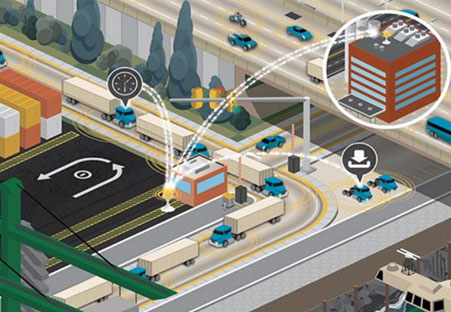
(Source: Federal Highway Administration.) In the remainder of this section, we discuss the inherent products of the transportation system and why they are as important as by-products in characterizing system performance—although they are often ignored or left as unquantified (and therefore unimportant) notions. The 21st Century analyst plays a key role in helping define, quantify, and estimate system products (and by-products) to inform a 21st Century concept of system performance. The Trap of Managing a System Using By-Products AloneBy-products of the movement of people and goods are inherently negative: e.g., crashes, fatalities, fuel consumed, and emissions. The by-products are no more (or less) important than system products. However, if by-products alone are used to characterize system performance, there are nuanced effects that can result in irrational investments. The problem of managing by-products alone is that any alternative examined that reduces system use is characterized as having at least some positive effect. Taken to an extreme, one can simply point out that a transportation system with no users has no negative by-products: zero crashes, zero fatalities, zero delay, and no environmental impacts. Clearly, this is a self-evident negative outcome, wherein the transportation system is completely unused and moves neither people nor goods. There must be some counterbalancing measurement of the system product so a more complete picture of system performance can be made. Even for cases less extreme than the "empty system," there can be subtle negative effects. Essentially, any considered alternative that suppresses use of the transportation system will accrue benefits associated with reduced by-products. Hidden deep within complex analyses, the benefits of improving system capability to reliably deliver people and goods are not valued—while small changes in delay and other by-products are measured, monetized, and used to inform decision-making. Why has system performance traditionally focused on system by-products? Simply put, it is because system by-products are easier to observe and measure than system products. When a crash occurs, it can be counted, as well as associated fatalities and delay measured or estimated. Legacy 20th century technologies (e.g., loop detectors) used to monitor a system are geared to provide snapshots of roadway speed, transit system ridership, and congestion. These systems only detect individual vehicles and travelers as indistinct entities. We may be able to count and classify vehicles by size, but only where we find them. The notion of the snapshot of conditions in time fails to reveal the reality of trip-making and goods delivery within the system. The 21st Century analyst can introduce a more balanced performance measurement approach, quantifying both products and by-products. Mobile phone technologies and wirelessly connected vehicles are increasingly capable of generating data that can quantify efficient trip-making within a network. Modern "smart tag" technologies associated with cargo can have a similar impact on characterizing both the volume and reliability of goods movement. Further, modern time-dynamic analytical methods can be used to characterize the amount and quality of mobility delivered by a transportation system, either as a part of a retrospective analysis or in the analysis of competing future alternatives. Managing System Performance: Maximize Products, Minimize By-ProductsA 21st Century characterization of managing a transportation system can be described as a two-ledger system wherein system products (people and goods delivered reliably) are maximized and system by-products (crashes, fatalities, delay, and environmental impacts) are minimized. Some agencies understand this important point and have begun to include mobility product measures as a part of their routine performance reporting. For example, Florida includes aggregate freight deliveries as a measure of performance in their performance indicators. (Florida Transportation Indicators.) Other agencies calculate broad annual estimates of economic impact, including access to jobs. The American Association of State Highway and Transportation Officials (AASHTO) New Language of Mobility (2013) (The New Language of Mobility: Talking Transportation in a Post-Recession World.) recommends AASHTO "green light" language for describing transportation system performance to the public, including sustainable mobility, economic impact, and access to jobs. However, these system product examples are far less prominent, less quantitative, less precise, and broadly aggregated in nature than associated by-product measures. The 21st Century analyst can bring data and tools together to provide increasingly robust and quantitative measures of system performance. Some useful measures of system products over a period of time (e.g., a peak period, or a day, or a month) include reliably completed trips and total value of goods delivered. While these products may be hard to measure directly, using time-variant travel time data and supporting estimates of ridership and volume data, the 21st Century analyst can conduct travel reliability analyses that are a key first step in the measuring a system product. Reliability data are a key element in characterizing trip-making since, if a trip takes much longer than expected, the disbenefits associated with disrupting travel plans outweigh the benefits. This is particularly true for goods movement within a supply chain, but the same basic principles hold for person-trips. For example, if a trip home from work takes longer than expected and a change to child-care arrangements is required, this can have direct and measureable financial consequences. The Congested Port Example Consider a collection of roadways connecting a port facility with goods distribution points in a large metropolitan area (see Figure 7). Access to the port facility may be plagued with unpredictable delays at certain times of day. To keep the port active and competitive with other ports along the seacoast, the region might consider a system that rations port facility access to reduce delays and make trips more reliable. Another alternative under consideration is to make a series of related capacity improvements at known bottlenecks in port access (e.g., freeway interchange movements, signal timing plans, and port-entry processing procedures). Data are then collected, and a well-constructed delay analysis is conducted. The Access Rationing alternative reduces delay by 35%, while the Capacity Improvement alternative reduces delay by only 7% (and costs more). Based on delay alone, a rational decision-maker would choose the Access Rationing alternative. An analyst could also calculate a measure of the number of containers reliably delivered in a peak three-hour period—a Peak Reliable Throughput measure. Using this measure, the Access Rationing alternative does not change peak reliable throughput while Capacity Improvement improves peak reliable throughput by 10%. Now the relative merits of the two alternatives can be weighed using a balanced discussion of a tradeoff in the economic benefits of higher peak throughput versus lower delays. It may even lead to a discussion of how a third alternative combining the most valuable aspects of both alternatives can be conceptualized and evaluated. Figure 7. Illustration. Example of a measuring system product.
(Source: U.S. Department of Transportation.) What Does "Good" Look Like—Multiple Stakeholders, Multiple ViewsUsing a balanced scorecard approach for performance measures can also help engage stakeholders in a discussion of what "good" looks like for a particular system. The 21st Century analyst has a key role to play here as well. If a high-level description of measures (e.g., delay or crashes) are listed on a single page, stakeholders and decision-makers only engage at the highest level in discussions of tradeoffs. When the time-dynamics of the system are explored in terms of more precise, quantitative measures, this sharpens the focus and discussion to reveal underlying differences in stakeholder viewpoints—viewpoints that very rarely represent a consensus. The analyst does not represent a specific viewpoint in this discussion; instead, he or she facilitates a reconciliation of give and take among stakeholders that can lead to a more informed, nuanced consensus about "good" system performance. This is critical, since if an analytic project is conceptualized, scoped, designed, and delivered with an underlying flawed conception of system performance, regardless of the technical skill of the analyst, the analysis will carry these flaws forward. These flaws can threaten the value of any analytic project, potentially increase analytical cost, and threaten the quality of any decision-making informed by such an analysis. Creating System Congestion, Reliability, and Safety ProfilesWith enriched data sources, time-variant profiles of key performance measures are indispensable for bringing depth and clarity to deliberations on system performance. Before jumping to scoping an analytic project, it is necessary to understand current system performance and review existing studies associated with the defined system. This step can lead to more effective analytical project development, more focused and valuable analytical results, and a more efficient use of resources associated with analysis. To start building system profiles, with identified problems and defined system boundaries (see the Introduction), data analysis is used to identify and collect/assemble the existing data and analysis results for diagnostics. The profiles include the data used in related (previous and current) analyses, the hypotheses and findings of these studies, and the insights gained by the analysts who conducted these studies. For example, an intersection with a high crash rate is identified within a transportation analysis. Before scoping a project to solve this problem, a data analyst pulls out the time-variant crash data at that intersection and searches relevant studies—such as intersection design studies, traffic signal design studies and crash attribute studies—to create the system profiles and document findings from the previous studies. Standardizing Methods for Performance MeasurementUsing existing information to identify/diagnose system problems, the system performance profiles are developed and maintained in a continuous process based on system management needs and the availability of data and tools. Performance measures should be consistent over time; within a day, month to month, or year to year. Standardizing how data are collected and processed is the key to ensure quality and consistency of performance measures identified in the system. Guide on the Consistent Application of Traffic Analysis Tools and Methods (FHWA, Guide on the Consistent Application of Traffic Analysis Tools and Methods, November 2011.) listed the main benefits of consistent analysis throughout the project development life cycle as follows:
Because the transportation system is in a constant state of change, we need to describe the system in a way that the performance measures and the methods by which those values are calculated are consistent, the measures are comparable, and how the system performs is consistently understandable over time. When a new data set or new sensors are added, data analysts need to revise the calculation methods so the new data can be added properly, and document the changes so a meaningful comparison can be made in the future. That way, when monitoring and diagnosing system performance, confounding factors can be eliminated to the minimal effect and the subjective performance measures can be evaluated constantly through and even beyond the project cycle. System ProfilesThe purpose of building system profiles is to characterize system performance (the system is getting better or worse) and to identify anything missing in the profile so the profile can be improved over the long term. With a large volume of data from different sources, using traditional data analysis techniques to develop system profiles can be cumbersome when an analyst attempts to find patterns in the data and establish relationships among variables. Using modern data mining and visualization techniques can lead 21st Century data analysts to insights that would be difficult to discover using traditional methods. This section offers a series of example system profiles (including their key components): congestion profiles, reliability profiles, and safety profiles. Congestion ProfilesTime-variant congestion measures may contain travel time, vehicle delay, bottleneck throughput, queue length, vehicle stops, and other attributes, depending on the nature of the problem and the system features. For example, to create a freeway corridor congestion profile, travel time and bottleneck throughput may be selected as performance measures; to analyze an intersection performance, queue length and vehicle delay may be used throughout the study. Figure 8 presents an example of congestion maps from Washington State Department of Transportation (WSDOT). (Traffic Map Archive.) Figure 8. Map. Washington State Department of Transportation congestion maps.
(Source: Washington State Department of Transportation.) Using speed data, WSDOT has archived a system-wide congestion map on ten-minute intervals since January 2013. These maps can be used in sequence in a simple and intuitive way to identify problem or bottleneck locations, as well as other changes within the system over time. Figure 9 illustrates another example congestion profile from the Kansas City Scout Traffic Management System (KC Scout). (Kansas City Scout Traffic Management System.) KC Scout developed a traffic dashboard to graphically display speeds and travel times by roadway segment in 15-minute, 30-minute, or 1-hour resolution. Figure 9. Snapshot. Kansas City Scout traffic dashboard.
(Source: Kansas City Scout.) Reliability ProfilesA within-day time-variant travel time chart is an effective way to convey system-wide or individual-route travel-time reliability. When combined with the number of delivered trips, the data can also be used to measure and report reliable throughput. The FHWA Travel Time Reliability Measures Guidance (Travel Time Reliability Measures Guidance.) suggests a set of performance measures used to quantify travel time reliability: 90th or 95th percentile travel time, buffer index, planning time index, and frequency that congestion exceeds some expected threshold (see Figure 10). According to the guide, travel-time reliability measures the extent of this unexpected delay and provides this definition: the consistency or dependability in travel times, as measured from day-to-day and/or across different times of the day. Figure 11 presents a plot of a within-day roadway segment travel-time distribution from Monday to Friday from KC Scout. The average and variation of travel time can be easily identified from this graphical expression. Figure 10. Chart. Reliability measures are related to average congestion measures.
(Source: Mobility Monitoring Program.) Figure 11. Chart. Roadway travel time distributions.
(Source: Kansas City Scout.) Safety ProfilesCommon safety measures include crash rates and number of fatalities, which can be acquired directly from state or local agency databases. Similar to a congestion profile, a geographic illustration can be an effective way to identify the problem locations. In the KC Scout Annual Report (KC Scout FY 2013 Annual Report.) (see Figure 12), KC Scout uses a heat map to illustrate the locations of multiple-vehicle incidents in 2013 to intuitively identify severe/high-incident rate locations. Figure 13 gives another example of geographically illustrating archived incident records from the Regional Integrated Transportation Information System (RITIS) developed and maintained by University of Maryland's Center for Advanced Transportation Technology Laboratory (CATT Lab). (University of Maryland CATT Lab.) Figure 12. Snapshot. Top multi-vehicle incident locations by route.
(Source: Kansas City Scout.) Figure 13. Snapshot. Maryland average annual incident frequency during morning peak hours by location.
(Source: Regional Integrated Transportation Information System.) Special Considerations for System ProfilesWhen creating system profiles, there are several considerations that require special attention to ensure that the data are treated properly and the resulting profiles are analytically sound. Additional discussion regarding the treatment and analysis of data can be found in Module 3. Inconsistent DataWhen preparing the system profile based on existing data and studies, analysts may face the situation that the relevant study data are neither comprehensive nor collected consistently over time. While data may be available on a subset of intersections, incident data may only be available for the past five years, and/or travel time data were collected before a new interchange was built. Data in these cases need not be thrown out—with some adjustment or identification of the limitations of these data, useful system profiles may still be constructed. Outlier EventsAbnormal traffic conditions due to outlier events (such as sports events or extreme weather conditions) cause bias if they are not separated from regular traffic conditions. Traditionally, these types of conditions are either averaged out in analysis or treated as outlier data and removed from the analysis. These types of operational conditions can actually be identified from different data sources using cross reference approaches (such as data mining) or statistical approaches (such as cluster analysis). Seasonality and Cyclical TrendsSeasonality is a pattern in time series data that repeats every year. This repetitive pattern in transportation can be attributed to a variety of causes. For example, an examination of monthly congestion data could offer a view of the systematic intra-year movement or seasonal patterns of congestion. There are variations in these patterns among different systems. These trends can be obtained by examining weekly, monthly, or seasonal averages of demand, congestion, and safety measures. Figure 14 illustrates an example of monthly travel-time reliability trends in the National Capital Regional Congestion Report. (National Capital Region Congestion Report.) Taking advantage of the availability of rich data and analytical tools, the Metropolitan Washington Council of Governments (COG) produces the quarterly updated traffic congestion and travel-time reliability performance measures to summarize the region's congestion and to examine reliability and non-recurring congestion. Figure 14. Chart. National capital region congestion report.
(Source: Council of Governments.) Preparing Predictive Profiles over Different Time HorizonsWith comprehensive information gathered, a data analyst can predict trends over different time horizons. In a short term, without changing system service (such as opening a new ramp or a new bus route, or starting new construction), the profile should remain the same or follow the previous trends. In the long term, statistical methods and transportation planning prediction models can help analysts predict the trends. Analysts need to highlight the changes and key factors influencing the performance measures and select appropriate methods to prepare predictive profiles. DiagnosticsHaving a set of relevant and dependable system performance profiles is a key resource for the 21st Century analyst to both understand patterns of system dynamics and to recognize when something new (and potentially problematic) is happening in the system. Much like a doctor takes measurements of a patient's blood pressure, pulse rate, and other data over time to establish a historical "healthy" range of vital statistics, the informed analyst has an analogous historical record of system dynamics to rely upon when assessing the nature, root causes, and severity of issues within the transportation system. Keeping data at a relatively disaggregate level is key in establishing what a consistent "healthy" range for these data may be. If we calculate an average blood pressure over two years, a doctor may find nothing of note. However, if an underlying pattern is changed (say the presence of some disorder), then blood pressure in the last two months may be much higher, falling outside a statistical range (e.g., a one-sigma band) taken using prior historical data. This is a clear signal to the doctor that something has changed, quite possibly for the worse, and that the system performance has deviated from previous patterns. In this section, we refer to diagnostics as the process where an analyst considers the set of historical system performance profiles to identify anomalous or problematic elements of current system performance. This diagnostic activity can be either direct or indirect in nature. Direct diagnostics occurs when an analyst engages directly with the data to make observations and hypotheses about the nature, root causes, and severity of system performance issues. Indirect diagnostics occurs when a stakeholder suggests an observation or hypothesis regarding system performance that the analyst may be asked to investigate. Both direct and indirect diagnostic activity are useful. A successful 21st Century analyst often finds highest value from a balanced slate of direct and indirect diagnostics. Direct diagnostics allows the analyst to develop new insights derived solely from the data. In some cases, no other stakeholder may be considering the full range of these performance data, and the analyst provides a valuable and unique viewpoint to inform system management. Indirect diagnostics can reveal important insights regarding potential issues in the system from stakeholders with different experiences in the system, and therefore different viewpoints that are not data-driven. These insights are nearly always valuable in their own way, and sometimes reveal limitations in the data quality, data coverage, and selected performance measures. System profiles, and system performance data, are not perfect indicators of actual system performance. Successful analysts fully engage with a set of stakeholders with different vantage points from which to assess system performance. If an analyst is disconnected from these stakeholders, the value of purely active diagnostics is lower because it is not informed, tested, or enhanced by these alternative viewpoints. Further, the analyst should keep in mind that data itself cannot always be an infallible barometer of system performance. The ways that data are collected, processed, and analyzed can always be improved. The remainder of this section presents tactical guidance on how the analyst can engage with stakeholders to leverage their insight, reconcile perception and observation, and create concise, targeted hypotheses regarding system performance. These hypotheses, when considered together, are the raw material used to generate preliminary analytic problem statements. Leveraging Data and Stakeholder InsightObservations about the performance of the system can come from many different viewpoints: from system managers who observe the buildup and dissipation of congestion through graphical displays and camera images, from agency staff who maintain the system, from the public safety officers who traverse the system, and from travelers themselves. When something isn't "right" or when system dynamics change, there are likely stakeholders within the system who notice that something out of the ordinary is happening. Whether this insight comes from direct, hypothesis-oriented engagement with data or the experience of observing or traversing the transportation system, it is important to establish processes and relationships that pull together insights from diverse stakeholders. The 21st Century analyst actively cultivates a set of performance-oriented individuals who engage with the transportation system in diverse ways. This cadre of contacts can provide invaluable observations that, when combined with data-driven observations from direct diagnostics, can lead to more substantive candidate hypotheses and ultimately more meaningful analyses. A hypothetical example where data-driven and stakeholder insight can be usefully combined is shown in Figure 15. Consider an analyst who notices a change in a reliability profile report covering the last quarter for northbound afternoon travel. This might be a one-time anomaly associated with a transient event (e.g., a temporary change in demand pattern), part of a longer-term persistent trend (e.g., the effect of new housing or employment center opening), or simply a misleading artifact related to erroneous data (e.g., loop detectors or speed sensors having been recently recalibrated). Around the same time, a staff person directing maintenance crews and pavement inspections notes that getting around the network in the afternoon in the northbound direction is more tedious than any time in recent memory, with longer and more unexpected delays. This same staffer observes that the pavement quality in some of the northbound sections has markedly deteriorated over the recent bitter cold winter months. The staffer might observe that something was amiss and might attribute the change to the pavement conditions but couldn't be sure since other factors (e.g., demand patterns, incidents, and weather patterns) might be in play. Independently, the two observations regarding the northbound system performance might be shrugged off or not considered critical or never brought together. However, just considering the two observations together proves much more powerful than if the observations were only considered independently. Figure 15. Flowchart. Leveraging direct (data-driven) and indirect (non-data) observations.
(Source: Federal Highway Administration.) In this regard, the two forms of observations can be powerful evidence when trying to pin down the nature, severity and root causes of poor system performance. Like a detective, the analyst can pull together independent observations to better establish the context for a particular issue and create a candidate hypothesis (see Figure 16). This doesn't mean that just because the analyst observed a change in travel-time reliability and the staffer wondered about the effect of the pavement conditions that we can immediately jump to the conclusion that there is a simple and straightforward reason for recent poor system performance. The analyst is still obligated to assess the validity of the underlying data to ensure that the change in system performance is not related to changes in data collection and processing. Many state DOTs with large loop detector systems perform routine validity checks on data quality to screen for issues, but the analyst cannot blindly assume that these are 100 percent effective. Figure 16. Flowchart. Cross-validating observations to create a candidate hypothesis.
(Source: Federal Highway Administration.) Reconciling Perception and ObservationCombining insights from individual observations and the analysis of data can lead to powerful and effective outcomes with respect to understanding system dynamics and developing candidate hypotheses. Figure 17 provides an example to how perception—supported by targeted data analysis—can lead to key insights regarding system dynamics and help to focus efforts to mitigate and resolve system performance issues. The "Underutilized" Arterial Example In an urban traffic management center several years ago, Transportation Management Center (TMC) staff had an excellent birds-eye view of a local freeway bottleneck from the windows of their facility (see Figure 17). Every day, they observed the buildup and dissipation of congestion where a major on-ramp fed into the freeway just ahead of a lane drop. Every weekday morning, congestion would develop at this location and stretch for a distance back onto the freeway, which was elevated from the surface street below. The arterial network in the vicinity was also visible to the TMC staff, and these roadways had no visible congestion; in fact, they appeared almost deserted in comparison with the densely packed freeway system. The TMC staff felt that if only the travelers knew how empty these surface streets were, they would flock to them, making use of the arterial system and freeing up the bottleneck on the elevated freeway. A data analyst working with the TMC staff had access to freeway counts and travel times but no arterial data. To better diagnose the nature of the "freeway bias" problem, a short-term travel-time study on the arterials was conducted to see how much travel time might be saved for popular origin-destination pairs along this part of the system. As it turned out, in the morning peak period, the travel times on the freeway, although at a slower speed, were quite comparable to the travel times on the arterial system. The arterial travel times were slowed both by signals and delay in accessing the surface street network from the elevated freeway system. In the end, the observed differential in vehicle density did not equate with a difference in vehicle travel time. The team then turned their attention to analyzing alternative methods of improving traffic flow in the bottleneck section, rather than on the provision of more detailed traveler information on changeable message signs. Figure 17. Illustration. Example of reconciling perception and observation.
(Source: U.S. Department of Transportation.) Preliminary Analytics Project StatementsThis section discusses how to characterize and categorize a list of hypotheses/problem statements developed from the diagnostics step, provide the possible strategies to fix the problem, and consolidate the analytics projects based on available resources. Characterize Problem Statement(s) and Identifying Candidate StrategiesWith the problems identified and verified from the system profiles and the hypotheses regarding the system performance developed from the diagnostics step, an analyst then tags the problems/hypotheses with attributes. The attributes may include system-level; location-specific or with geographical constraints; temporal; with certain conditions; dealing with certain conditions, such as work zones; and dealing with certain improvements, such as traveler information. Some problems/hypotheses may be well defined (like a bottleneck at a weaving area), and some may be more generic (such as system travel-time reliability). Each of the problems/hypotheses can be assigned to one or more analytics projects. From the hypotheses, an analyst merges some hypotheses together if they are related or break down into some subsets if the hypotheses are system-wide. For example, there is a bottleneck on a freeway segment. From diagnostics, the bottleneck occurs during peak hours due to the large merging and diverging activities at the weaving area. This is a well-defined problem/hypothesis with clear attributes. The problem could be a stand-alone project or could be combined with other problems with the similar attributes, such as the timing issue of the ramp metering near the bottleneck location or the traffic signal optimization issue at the interchange near the bottleneck location. To form a problem statement for an analytics project, the next step is to add possible strategies to fix the problem (alternative identification); possible approaches/methodologies to analyze the problem, (e.g., simulation or field test), and data needed to conduct the project. To solve the bottleneck issue at the freeway weaving area, a simulation model may be needed to evaluate all possible alternatives, such as adding one auxiliary lane, creating a Collector/Distributor (CD) lane, or optimizing the on-ramp metering with a new set of optimization criterion that takes into account the freeway throughput or speed. An analyst could suggest performing a field test on the later strategy but not on the first two strategies due to the risk and cost-effectiveness issue. Some of the strategies might be developed by the analyst and some of the strategies may be already suggested by the stakeholder at the diagnostics step. Using the bottleneck at the weaving area as an example, Table 1 presents a hypothetical example of initiating a problem statement. Consolidating Analytics ProjectsA key role for the 21st Century analyst revolves around deriving ideas from their own direct observations, talking to the stakeholders, and sorting things out. A purely passive stance of waiting for problem statements to come from stakeholders is not recommended because this may yield a set of incremental or partial concepts that may be individual facets of a larger problem. One major contribution from the 21st Century analyst is to consolidate analytics projects, where several small issues can be grouped and analyzed together to better use resources and gain a better value. For example, pedestrians crossing an intersection, lack of progression at an arterial and a rise in unprotected left-hand turns mid-block on the same arterial can be consolidated into one project or related projects that can share resources and maximize the system performance. Another key item an analyst needs to guide the selection of which analytical projects to move forward with is a high-level technical risk and reward (value) analysis for each candidate project before prioritizing the problem statements. Risk AssessmentAn analyst considers all the possible strategies to provide a high-level technical risk assessment, resulting in a rating of low, medium, or high. Risks could be related to the size of the network, the availability of supporting data, or the complexity of the most appropriate analytical methods. Risk is related to all the things that can make doing the analytics work difficult, costly, or create the potential for technical failure. The following bullets are some examples to be considered:
Value AssessmentSimilar to risk assessment, an analyst lays out all values/benefits from each analytics project ranging from low to medium to high. The values include immediate values and potential or long-term benefits. The following are some examples for consideration:
Risk/Reward AssessmentA simplified risk/reward assessment could be conducted to help the later prioritizing step. Moreover, it could be another way to group some projects with low risk and low values if the combination produces higher benefit due to the natural relations between the projects. Figure 18 illustrates a simplified version of a risk-reward assessment chart where the identified projects are placed in one of the boxes to address the risk and reward based on the list of the risks and the values listed above. Figure 18. Chart. Risk/reward assessment chart.
(Source: U.S. Department of Transportation.) Where Transportation Analysis Provides Unique ValueSome straightforward problems can be done by pure retrospective data analyses or by conducting a simple field test. Other problems may involve multiple strategies that cannot be tested in the field and require a modern simulation technique to evaluate the strategies—or a hybrid approach using a small-scale field test to verify the values of the parameters and input the observed data into a virtual network to simulate possible strategies. The 21st Century analyst has a valuable and unique insight into system dynamics, underlying system issues, and potential mitigating strategies. The analyst also brings an understanding of where data alone may be able to answer critical questions and when more complex modeling may be required. These are critical insights into making resources deployed in analytics less risky, more accurate, and more useful. Prioritizing Analytic Problem StatementsOne key step in getting the highest value from analytical resources is making strategic decisions on which analytical ideas to move forward and scope as projects. We recommend doing this periodically, considering a complete portfolio looking across all the candidate ideas generated, rather than individual projects one at a time as the ideas come up. This may not always be possible—in some cases, urgent needs may arise off-cycle that must be dealt with individually. However, a process that is purely reactive runs the risk that high-value analyses do not have resources available because lower-value projects have already claimed all available analytical resources (staff time and budget). Figure 19 illustrates a portfolio of ten potential analytical projects considered within a portfolio analysis. In this case, the analyst has rated each project as LOW-MED-HIGH on each of the two assessment axes (RISK and VALUE). Clear winners to move ahead include Project D (High Value, Low Risk), Project G (High Value, Medium Risk), and Project J (Medium Value, Low Risk). Possible projects to consider include Projects I, E, F, and B, where risk and value have equivalent assessment ratings. Projects A, H, and C are not good candidates because each has higher risk ratings than value ratings. Figure 19. Chart. Risk-reward assessment of candidate analytical projects.
(Source: U.S. Department of Transportation.) The process of optimizing a portfolio of analytical efforts is the next step in the process. The goal is to commit resources to scope only the highest value collection of potential projects while minimizing risk. While pure optimization methods do exist for portfolio analysis, in this case, our recommendation is for a qualitative prioritization using the gathered information rather than a strict quantitative optimization. At this point, we are not committing funds to conduct the analysis, we are only moving forward a set of promising candidates to formal scoping. Why do we limit the number of projects to scope? Because even at this preliminary level, the effort to scope a project effectively is not trivial. In fact, a common trap for analysts is to have many analytical project concepts then try to jump directly into preparing a formal data collection plan and full analysis plan. This aggressive form of project development is problematic on two fronts. First, key details of the analysis have not been completely thought through, so there is a good chance of wasted effort in data collection and in the analysis phase. Second, the resources incurred to prepare a detailed plan may be wasted when at some point in the effort it is determined that the project is too large, too risky, or infeasible for various reasons that would have surfaced in a formal scoping effort. The goal is to choose a focused number of high-value projects to move forward into scoping, and to allocate sufficient resources and attention to these projects so they are properly and thoroughly scoped. Consider a total analytical budget representing some combination of staff time, staff experience, and budget available in this round of projects selected for scoping. Clearly, this is not an unlimited resource. The analyst assesses the effort associated with thoroughly scoping each of the projects in terms of HIGH, MEDIUM, and LOW effort. Taking these into consideration, the analyst identifies the target number of projects that can be well-scoped in each category, say one HIGH, one MEDIUM, and two LOW projects. The prioritization process begins by selecting the project with the highest value over risk rating. In our example, this is project D, with HIGH value and LOW risk. Assume this is a MEDIUM effort project, and it takes the MEDIUM slot in the available scoping portfolio. The next two high-value projects (J and G) are rated HIGH and LOW effort for scoping and take the next two slots. Among the remaining moderate value/risk projects (B, E, F, and I), the analyst should choose among projects rated as LOW effort. As discussed above, this process is qualitative, not strictly quantitative. If there are two HIGH value/HIGH effort projects, the analyst may decide to pursue the second HIGH effort scoping in lieu of the one MEDIUM and two LOW efforts. The goal is to make this process systematic and clear but not so inflexible that low-value/risk projects are consistently selected over higher value/risk projects. The process can also be documented so that all stakeholders have buy-in on the portfolio of projects selected for scoping. Another consideration at this phase is that just because there are analytical resources to move forward with these projects, are they worth moving forward? Just because staff time or funding is available, low-value, high-risk efforts may not be good analytical investments. At this point, the analyst should be cognizant that it may be time to identify new project ideas or to modify the current ideas so they can be more valuable and/or less risky. Moving to Module 2: The Analytic Problem StatementIn order to move to Scoping (Module 2), a minimum set of information generated in this step of the process needs to be documented for each project as an analytic problem statement. As indicated in Table 2, this can be represented in a single page.
These problem statements are a critical resource for improving the analytical process over time. The analyst can demonstrate stakeholder engagement and involvement. Early statements can be compared against completed projects to assess the accuracy of initial estimates of effort, risk, and value. This can prove invaluable in improving the quality of early project identification over time and can help focus resources on the most critical near-term projects. To some, the development of problem statements and performing a risk/reward analysis may not seem like time well spent—perhaps the time could be better spent running models and grinding up data. In fact, this early process of diagnostics and systematic problem statement development may be the most critical element of creating a more efficient organization-wide analytical capability. The amount of effort is low; it is essentially a bare-bones effort to document a process that occurs in an ad hoc fashion in many organizations. When a project idea is identified, the person with the greatest insight may not be there when the project is scoped, data collected, or analysis performed. The insights must then be documented so that the original intent of the work (as defined by the stakeholders) is not lost. Otherwise, there is a risk that a different, lower-value, higher-risk effort is scoped and performed—all because of a lack of documentation at this early stage. You may need the Adobe® Reader® to view the PDFs on this page. |
|
United States Department of Transportation - Federal Highway Administration |
||