Measuring the Impacts of Freight Transportation Improvements on the Economy and Competitiveness
4. Tools and Techniques
This section discusses three types of analyses that may be used to consider the impacts of freight transportation projects: benefit cost analysis (BCA), economic impact analysis, and regional productivity (competitiveness) analyses. A discussion of the goals, basic methods and tools available for each of these analytical frameworks follows. It is important to note that discussion of these tools does not provide an endorsement for any specific software tool or approach. This section provides an introduction to tools and methods that are available and in-use, but users will need to make their own evaluation to determine if any of these approaches or tools meets their needs.12
4.1. BENEFIT COST ANALYSIS
The BCA is an important tool for planners to determine whether investments in transportation infrastructure are economically and socially beneficial. It provides a standardized method for policymakers to assess the value of different types of benefits occurring at different points in time. Conducting a BCA is one way for planners to view the benefits and costs of transportation investments from a more global and all-encompassing perspective, rather than just looking at local impacts. In addition, by making the assumptions and analyses of public sector agencies more explicit, BCAs can help public-sector agencies communicate their planning perspectives to the stakeholders in the planning process.
4.1.1. RELATIONSHIP OF TRAVEL DEMAND MODELING TO BENEFIT COST ANALYSES
Travel demand modeling serves as the foundation for many BCAs, particularly for larger projects that will cause regional effects on traffic. The outputs of travel demand models provide estimates and forecasts of highway performance measures under different scenarios. These include forecasts of traffic volumes, travel time, and delay by segment, which are the basis for estimating the benefits of different investment scenarios. Because of its importance, below is a brief overview of travel demand modeling and its relationship to the BCA.
In order to plan for future transportation needs, regional transportation planners typically use a four-step travel demand model to estimate future volumes of trips on the transportation network. The four steps are trip generation, trip distribution, mode choice and network assignment. These four steps predict where trips will be coming from, where they will be going, what kind or transportation they will use, and what specific route they will use.
In the trip generation phase, planners estimate how many trips originate in each traffic analysis zone using data on the demographic characteristics of the population. For freight trips, surveys, models, and economic data can be used to forecast truck trip or freight generation, although acquiring this data may require significant effort.
Figure 1 below shows different approaches to incorporating freight trucks into transportation demand modeling. Our focus here is on modeling at the State or regional scale, since these scales are most typically associated with using travel demand models to estimate the benefits of specific projects. The approaches include estimating a commodity freight table synthetically (step 4), using acquired commodity flow tables (step 6a), using a separate service truck model (step 8), or using economic modeling approaches that use economic or land-use activities as exogenous variables to estimate freight flows (step 6b). Each of these approaches to estimating freight movement or truck trips would serve as inputs into different places in the four-step modeling process. NCFRP Report 8 – Freight Demand Modeling to Support Public-Sector Decision Making13 provides more context for the overall framework and each of these approaches, as well as additional detail on other models.
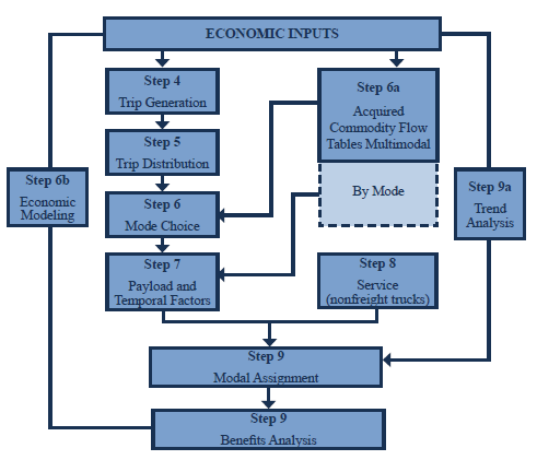
A number of the approaches discussed above bypass some of the steps of the traditional four-step model. When planners use a synthetic freight table, the remaining steps will occur (distribution, mode choice, assignment). In the freight distribution phase of the four-step process, the model estimates the distribution of freight flow ends. Based on distance and industry employment (or in some cases land use characteristics), the travel demand model estimates what percent of freight moves in each zone will be attracted to other zones. Although there are other methods, the distribution phase typically relies on a gravity model, which is a statistical model that estimates the geographic areas that will attract freight and how much they will attract. As noted in NCFRP Report 8 – Freight Demand Modeling to Support Public-Sector Decision Making:
In the gravity model for freight, as in other transportation applications, the mathematical equations used are applied separately for flows with similar behavior (e.g., commodities).The productions and attractions by commodity are distributed in the gravity model based on the accessibility between the zones, as measured by the impedance between zones. For freight models, the impedance variable for the large geographies considered by freight is most often found to be distance. By examining the commodity flow survey data, it is possible to determine those parameters, such as the average trip length by commodity, which are used to vary the accessibility in response to changes in the impedance variable.15
The mode choice phase of the model estimates which mode (highway, rail, other) that freight will use in moving between different traffic zones. Mode choice for freight depends on the characteristics of the mode, commodities, production zone, and attraction zone. Data sources such as the Commodity Flow Survey (CFS) can be used to estimate State mode choice models, but these models will be less accurate at the regional level where access to intermodal transport options may differ. Where insufficient data exists to properly model this choice, the future choice of mode can be assumed to be the same as the existing choice of mode. The Freight Analysis Framework (FAF) can be used to estimate changes in mode share in the future due to changes in the mix of commodities. For truck freight, tonnage flows need to be converted into truck trips using estimates of payload and temporal factors. Since medium- and heavy-duty trucks take up more roadway capacity than passenger vehicles, truck trips need to be converted into passenger equivalent trips.
The final phase of the model, network assignment, assigns each trip to a particular network route (Step 9 above). The truck origin-destination trip tables are combined with passenger trips before being assigned to the transportation network. Travel demand models can assign all of these trips to the network to estimate the routing of trips, changes in congestion, delay, and vehicle operating costs. These changes in system performance then serve as the inputs to a BCA to analyze freight transportation system improvements.
For both auto and truck trips, the model takes into account how congested each link in the road network will be. The model may divert traffic to less congested segments if high traffic volumes on particular segments cause congestion.
The four-step modeling process provides forecasts of travel activity that are important to determining the costs and benefits of a transportation improvement. Travel demand modeling provides forecasts of the number of trips occurring on the transportation system. This determines the universe of trips that might benefit from a specific improvement.
The model also takes into account the dynamic nature of travel demand. One can use a travel demand model to determine the level of demand for a roadway with or without an investment that improves the roadway. A transportation improvement may cause users to divert to improved roadway segments. Travel demand modeling seeks to estimate the volume of traffic that will be diverted. Traffic diversion may reduce the benefits of the transportation improvement to existing users, but it will also create benefits for users on other segments of the transportation network.
Travel demand modeling may also seek to estimate the changes in travel behavior caused by a transportation improvement. For instance, a roadway improvement may create additional trips or move trips into peak traffic hours if the investment reduces congestion. Travel demand modeling can estimate the effects of these behavior changes on the benefits of a transportation project.
The outputs of the four-step travel demand modeling process provide some of the inputs to a BCA. Travel demand models can estimate travel speed, delay, transit time, and traffic volumes on a transportation network. This can be done with and without a planned transportation improvement, providing data on a baseline and alternative transportation scenario.
It is important to note that travel demand models do not typically allow the user to separate passenger and truck trips after they have been assigned to the network. As such, a planner must make assumptions on how the overall changes in congestion and transit time measured by the model would apply to freight trucks.
Traditional four-step travel demand models have several additional limitations. Freight trip making is driven by a variety of factors that are not typically captured. For instance, the number of truck trips is determined in part by complex logistical decisions – the use of inventory, the frequency of shipments, the choice of equipment type, the average payload carried, vehicle repositioning, empty mileage, the location of warehouses, the choice of less-than-truckload or truckload shipments, vehicle routing choices, and other factors. More sophisticated models need to be used to more fully capture transportation and logistics decisions. Some of these microsimulation and agent-based models are briefly described below.
Other limitations of using traditional transportation demand models for freight is that they may not incorporate appropriate constraints for truck routes, time of day operating patterns, or geometric limitations for truck operations, nor may they reflect appropriate seasonality patterns in shipment deliveries.
It is also important to note that the four-step travel demand models typically only incorporate direct user benefits into their calculations. Broader secondary impacts or benefits derived from productivity improvements would require additional analysis techniques to estimate (discussed below).
Microsimulation Models and Agent Based Models
The traditional four-step modeling approach has difficulty capturing the factors that influence shipper and carrier behavior. Although more common for forecasting passenger travel demand, examples of freight behavioral modeling remain relatively limited. Microsimulation models represent the individual movement of large numbers of shipments and their attributes. Agent-based modeling defines potential actors in freight transportation. Each actor has an allowable set of actions and interactions. These models allow planners to perform "what-if" analyses and develop scenarios to understand the behavior of the freight system. More complex models can capture multi-stop freight delivery routes and represent more complex logistics, such as the movement of goods from warehouses and distribution facilities. As an example, larger transportation planning agencies in New York and Chicago have invested in these models. The Freight Activity Micro-simulation Estimator (FAME) is an example of a modeling framework that incorporates behavioral elements that can capture more complex logistics.16
FAME includes five modules to more accurately characterize freight transportation and logistics decisions:
- The first module recognizes all the firms in the study area and identifies their basic characteristics;
- The second module determines the types and amounts of incoming and outgoing goods based on each firm's characteristics and replicates their supply chain designs;
- The third module defines shipment sizes based on the previously collected data about the firms' characteristics and the way they trade commodities with each other;
- The fourth module makes decisions regarding shipping mode, haul time, shipping cost, warehousing, etc.; and
- The fifth module investigates the impacts of the movement of goods on the transportation network.
Regardless of how transportation impacts are estimated, the BCA translates the transportation impacts of various project alternatives into monetary impacts. The BCA provides a methodology for comparing projects with differing cost structures and benefit streams over time. It translates the impacts of these projects into net-present-value estimates and benefit-cost ratios that can be used to assess these projects both relative to a baseline case and against each other.
4.1.2. PURPOSE OF BENEFIT COST ANALYSIS
A BCA has three primary functions. First, it can be used to evaluate whether a project should be undertaken. It can answer the question "Will the benefits of a project exceed its costs?"
It can also be used to determine when a project should be undertaken. For instance, if a project is not currently beneficial, will traffic growth make conducting a project economical at a future date?
Lastly, the BCA can be used to identify which alternative should be funded. In many cases there are numerous projects that could be conducted to improve the transportation system. BCA can be used to answer the questions "Which alternative will yield the most net benefits?" and "How does a specific project compare to other projects that could be undertaken?"
4.1.3. COMPONENTS OF BENEFIT COST ANALYSIS
The major components of a BCA include the following: establish objectives, specify assumptions, define a base case and alternatives, analyze traffic effects, estimate benefits and costs relative to the base case, compare net benefits, rank the alternatives and make recommendations. Each of these is addressed in more detail below.
Benefit Cost Analysis – a Long and Wide View
"Benefit cost analysis is a practical way of assessing the desirability of projects, where it is important to take a long view (in the sense of looking at repercussions in the further, as well as the nearer future) and a wide view (in the sense of allowing for side-effects of many kinds on many persons, industries, regions, etc.), i.e., it implies the enumeration and evaluation of all relevant costs and benefits."
— Ken Button, Benefit/Cost Analysis for Transportation Infrastructure: A Practitioner's Workshop, Workshop Proceedings, August 2010
The first step in a BCA is to establish the objectives of the project. Objectives might include reducing congestion (by eliminating a truck freight bottleneck for instance), improving connectivity (by investing in a freight intermodal connector), or improving safety (by enhancing roadway geometric design to facilitate heavy-duty trucks). By clearly defining the objective, the number of project alternatives considered can be reduced.
Any BCA analysis will also rely on a set of assumptions. These would include assumptions about expected future traffic growth in the region over the life of the project and the likely composition of the future vehicle fleet. Forecasting future freight flows is more complex than passenger trips since freight movements are determined by global supply chains that are constantly shifting. Often a significant portion of freight traffic takes the form of external trips that are generated by production and consumption decisions occurring outside the region being studied. In addition, many truck carriers operate trucks that are registered outside of the region, making it more difficult to characterize the on-road fleet. The assumptions for a BCA might also include natural, legal or policy constraints on what projects can feasibly be undertaken.
Based on the objectives and the assumptions identified, a BCA analysis develops a set of alternatives to be assessed. Typically a baseline alternative that involves not undertaking an improvement (apart from providing routine maintenance) is identified. A set of alternative transportation improvements that could be undertaken are also specified and compared to the baseline. Improvements to the base case could include a rehabilitation or reconstruction of the existing facility to support heavier vehicles, the replacement of current infrastructure with a higher volume facility, or the addition of capacity to relieve congestion, such as or the addition of a truck climbing lane. Investments in eliminating impediments to the operation of heavy vehicles such as bridge clearances or turning radius restrictions could be studied. Improvements might also include operational investments, such as signal timing, weigh-in-motion technology, or other automated enforcement equipment that enhance the throughput of existing facilities.
In order for alternatives to be compared on a level playing field, the costs and benefits of each alternative (relative to the base case) need to be compared over their full lifecycle. A multiyear analysis period for comparing the costs and benefits of alternatives is established. Ideally, this analysis period should be long enough to incorporate a major rehabilitation activity for each of the alternatives.
Steps in a Benefit Cost Analysis
- Establish objectives
- Specify assumptions
- Define a base case & alternatives
- Analyze traffic effects
- Estimate benefits and costs relative to base case
- Compare net benefits and rank alternatives
- Make recommendations
The level of effort expended on a particular BCA should be proportional to the size and importance of the project. When a project is expected to generate significant benefits or have a major impact on relieving congestion, a BCA should explicitly analyze the traffic effects of the facility. Major improvements in transportation facilities can be expected to create substantial new demand, and a comprehensive BCA analysis should consider the effects of this new demand. Changes in future traffic volumes can be expected to alter the costs and benefits of the project.
The costs and benefits of an alternative are measured against the base case. Construction costs, delay costs, transit time benefits, crash costs, vehicle operating costs, emissions costs and others are measured by year and converted into a dollar value. The cost of delay to heavy-duty trucks is higher on average than other vehicles. The Federal Highway Administration (FHWA) uses $31.44 per hour for the average cost of delay for a five-axle combination truck while a medium auto has a delay cost of $16.92.17 The American Trucking Research Institute estimates the average cost of truck delay to be higher at $65.29. These estimated costs include the direct cost of operating the vehicle. Research on trucking has shown that shippers and carriers can value transit time as high as $200 per hour, depending on the product being carried. The value of reliability (i.e., the cost of unexpected delay) for trucks is another 50 to 250 percent higher still.18
A BCA considers an array of benefits and costs. Agency costs include design and engineering for a project as well as land acquisition and construction costs. Multi-year costs such as maintenance are also included. The construction of a project can also impose user costs as well. For instance, work zones can cause delay or increase vehicle operating costs during construction. In addition, crash risk may be elevated in work zones.
User costs and benefits include changes in travel time, delay and reliability. Reliability is often measured as the variance around either the transit time or average delay time.19 Truck carriers and shippers can build time into their delivery and ordering schedules to account for delays caused by recurrent congestion (such as rush hour delays). Unexpected delays caused by non-recurrent congestion are more costly. The value of reliability can be difficult to estimate for truck freight, since different types of commodities may have significantly different costs of delay associated with them. A manufacturing customer using a just-in-time delivery system may need to shut down their operations if they exhaust the supplies that are available for production. These types of shipments could incur very large delay costs. Shipments that are less time sensitive might have much lower delay costs associated with them. Unexpected delay costs have been estimated to be between 50 percent and 870 percent the value of truck delay time.20
Increases in crashes are also user costs. Typically travel time improvements create most of the benefits associated with a transportation investment. Travel time improvements are typically monetized using data on the average salary and overhead costs of workers. FHWA has recommended using an average value of $25.75 for truck drivers in Federal BCAs, and personal travel time is typically valued at 50 percent of the per hour median household income in the region. FHWA has recommended values for use in Federal Transportation Investment Generating Economic Recovery (TIGER) Grant applications that are broken down between personal and business travel, and estimated separately for local and intercity travel. For instance, they estimate that local personal travel time is valued at $12.42 per hour for surface transport.21 Projects to improve freight movement can have significant non-freight related benefits. For instance, an investment in an important highway freight corridor will also incur significant benefits from savings in passenger travel time as well.
Crash costs can be estimated using data on how much individuals are willing to pay to reduce their risk of an injury or a fatality. Default values for many of these parameters are available from a number of guidance documents discussed below. As would be expected, truck crashes tend to incur more costs due to the greater likelihood of severe injuries or death. FHWA uses $9,200,000 as the estimate of the value of a life. The TIGER Benefit-Cost Analysis Resource Guide provides estimates to value crash injuries of different severity levels.22
Externalities, or costs to non-users, are also considered by BCAs. Externalities are uncompensated impacts that are created by users of the system but that fall on others. Emissions, noise, and other environmental impacts typically impose costs on the public at large. Reducing the cost of externalities can be an important rational for investing in freight projects since freight contributes disproportionately to air emissions and serious crash injuries and fatalities. Trucks are a large source of air pollution in cities. Concentrated truck activity in areas that surround freight centers (e.g., ports) or freight-heavy corridors (e.g., freeways such as I-710 in Los Angeles) creates negative health effects in surrounding neighborhoods.23 A BCA monetizes these costs and includes them in the analysis. The U.S. Department of Transportation's (USDOT) TIGER Benefit-Cost Analysis Resource Guide provides methodologies and data to value criteria air pollutant and carbon dioxide emissions.
In a BCA, future benefits are discounted to a present value amount. Thus multiyear cost and benefit streams are translated into a single "net present value" that provides a measure of the value of the project. When discounted benefits exceed discounted costs, a project can be considered worth pursuing. One can compare alternatives against each other according to their net present value or their ratio of benefits and costs. The project that produces the greatest net present value can be considered the most economically valuable.
BCA identifies the projects or project alternatives that produce the greatest economic value or have the greatest ratio of benefits to costs. The results of BCA can be used to recommend projects that will employ resources in the most economically efficient manner, although policy makers may face other constraints, such as budgetary considerations, that should affect the selection of a project.
4.1.4. BENEFIT COST ANALYSIS TOOLS
A variety of software tools are available to conduct BCAs. These include MicroBENCOST, StratBENCOST, the Strategic Transportation Evaluation and Assessment Model (STEAM), BCA.Net, Highway Economic Requirements System State Version (HERS-ST), Intelligent Transportation Systems Deployment Analysis System (IDAS), GradeDec.Net and Cal-B/C. These tools allow the user to estimate the direct benefits and costs that accrue to truck operators, but do not estimate the indirect cost of congestion to freight shippers, who may incur additional inventory, production or other costs associated with the impacts of congestion on freight transit time or transit time variance. MicroBENCOST implements the American Association of State Highway and Transportation Officials' (AASHTO) guidance on conducting BCA described in A Manual of User Benefit Analysis for Highways. The program is capable of analyzing seven categories of projects: added capacity, bypass, intersection/interchange, pavement rehabilitation, bridge, safety, and highway-railroad grade crossing. The tool requires the user to input the percent trucks and the estimated composition of the vehicle fleet. While MicroBENCOST is not a freight-specific BCA tool, it provides the capability to analyze seven categories of improvements that will benefit both trucks and autos, such as truck climbing lanes.
Although MicroBENCOST is not commonly used, it is still distributed online in 201524 and updated guidance for its use in Canada was made available in 2014.25
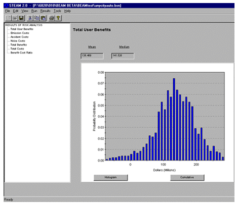
STEAM was developed by FHWA to estimate user benefits, costs, and externalities of transportation projects based on trip tables and networks from four-step travel demand models. STEAM calculates user benefits based on changes in consumer surplus for travelers at the link level. Figure 2 shows an output screen from STEAM. Transportation system alternatives may include up to seven modes. Peak and off-peak periods are also considered. Note that since STEAM is a post processor to travel demand models, a multi-modal transportation demand model is required to conduct multi-modal analysis. Similar to the other traditional BCA models discussed here, STEAM incorporates trucks by estimating only the direct benefits to truck operators and not the secondary benefits that may accrue to shippers.
StratBENCOST calculates benefits from time savings, vehicle operating cost reductions, accident-cost reductions, and emissions reductions. Similar to other software, benefits are calculated year by year in dollars, discounted to present value and summed.26 StratBENCOST provides two separate models. One model can be used for network analysis and can incorporate the outputs of four-step travel demand models. The second model included in StratBENCOST can be used for single segment analysis and is for individual projects that will not have network effects. StratBENCOST incorporates cost calculations from MicroBENCOST and HERS, and provides the additional ability to consider risk and uncertainty. The benefits and costs to trucks can be incorporated by manipulating the percent trucks input. Similar to the other models discussed in this section, only the direct costs and benefits to truck operators are considered.
BCA.Net is FHWA's free, web-based tool for conducting a BCA.27 The tool compares and evaluates alternative highway improvement projects (e.g., preservation, lane-widening, lane additions, new alignments, addition of traffic control devices, intersection upgrades). BCA.Net can evaluate multiyear, full-lifecycle investment and maintenance strategies. The model allows inputs for time-of-day distribution of traffic (e.g., peak, peak shoulder, off-peak) and traffic mix by vehicle type (e.g., auto, truck, bus). Benefits include time savings, operating cost savings, accident reductions, and air emissions reductions. BCA.NET allows the user to generate point estimates, or use risk analysis techniques to generate probabilistic results. One benefit of using this tool for freight analysis is that it allows the user to specify with some detail the percent of trucks in the traffic mix over time.28
HERS-ST is a State-level version of the Highway Economic Requirements System. HERS-ST can assess transportation investments targeted at pavement, geometric or capacity deficiencies. HERS-ST can estimate the highway system performance that would result from various transportation investment funding levels. While HERS is not focused specifically on freight, the model provides different operating costs and benefits for different vehicle classes, including heavy-duty trucks that are used in freight movement.
Some BCA software is tailored to particular types of highway investment. For instance, IDAS is used to assess the costs and benefits of ITS improvements. GradeDec.Net is a Federal Railroad Administration model that is used to assess benefits and costs of investments in highway-rail grade crossings. For instance, it can assess upgrades, grade separation and closures to highway-rail grade crossings.
CAL-B/C is a spreadsheet benefit cost model developed by Caltrans to conduct analysis of projects in the State Transportation Improvement Program and has been used extensively in the State. The tool can prepare analyses of highway, transit, and passenger rail projects. Users input data defining the type, scope, and cost of projects. The model calculates life-cycle costs, net present values, benefit-cost ratios, internal rates of return, payback periods, annual benefits, and life-cycle benefits. While the original Cal-B/C model focused on capacity expansion projects, subsequent versions have incorporated additional project types, including transportation management systems and operational improvements. The latest revision also expands the Cal-B/C framework to include companion tools that support link and network analysis, called Cal-B/C Corridor and Cal-NET_BC.29
The Highway Freight Logistics Reorganization Benefits Estimation Tool is different from the traditional BCA tools described above. The tool does not replace, but rather supplements, a conventional BCA by providing an additional analysis to complement a BCA. It relies on the data collected for, and output by a traditional BCA, for its inputs. In addition, the tool requires a conventional BCA where explicit freight-associated benefits have been calculated.
The Highway Freight Logistics Reorganization Benefits Estimation Tool calculates long-run benefits to the economy additive to the user benefits typically calculated in a benefit-cost analysis resulting from a highway investment. These benefits include reduction of shipping and sourcing costs, replacement of inventory on-hand with just-in-time delivery of inputs, and wholesale reformation of the supply chain. The long-run benefits estimated result from an expansion of markets and the shift outward in the demand curve for freight transportation. The tool captures the benefits that accrue to businesses and the economy as lower freight transportation costs allow businesses to reorganize their supply chains.
The size of the long-run benefits estimated by the tool will vary with project size and freight significance. Segments with minor performance improvements in non-freight significant corridors would create few long-run benefits from logistics reorganization. Segment improvements in freight significant corridors that can improve the reliability of delivery at key points would have more substantial long-run benefits. The greatest benefits would be expected where sizable networked corridor investments improve service for geographically distributed points. When investment improves transportation performance in corridors that meet the needs of diverse and numerous supply chains, large long-run benefits can occur. In these cases, logistics managers would have an incentive to adjust their supply chains, improving productivity and increasing the long-run demand for freight transportation through the corridor.
The key inputs to the Highway Freight Logistics Reorganization Benefits Estimation Tool are the baseline initial conditions, which include the project location, project length, baseline truck traffic, average effective speed, value of time, vehicle operating costs, and travel time reliability. The user also enters information on the effects of the proposed improvement, including changes in vehicle operating costs, travel time, and reliability. The user also enters the freight specific benefits from a traditional BCA. Based on these inputs, the tool estimates the reorganization benefits. This tool helps analysts using traditional BCA to incorporate the benefits that accrue from supply chain reorganization that enhances productivity. The tool is available for free on the FHWA website.30
Another important set of tools that can help in assessing the productivity impacts of transportation investments are those developed under the Strategic Highway Research Program (SHRP) 2 Capacity program. The SHRP 2 C11 project developed a set of spreadsheet tools to estimate the wider benefits of transportation investments. These tools are meant to be used in the "middle-stage" of project development, where a full blown analysis does not need to be conducted, but sketch planning is used to develop an improved understanding of what the magnitude of benefits for investment might be. The SHRP2 C11 tools "shift the focus of analysis from traditional transportation impact measures (i.e., travel time, cost, and safety) to broader factors that also matter to individual business operators and thus actually 'drive' economic development processes (i.e., travel time reliability, intermodal connectivity, and market access)."31
SHRP 2 C11 Reliability Tool – Improved transportation reliability allows business to reduce the cost of logistics. Reducing late deliveries enables a reduction in inventories (safety stocks) and can allow more centralized warehousing and delivery processes to be put in place.32 The reliability tool takes information on the type of highway, projected traffic volume, speed, lanes and capacity, and generates measures for travel time index, average delay, buffer time, and cost of delay. The travel time index and buffer time provide a basis to further calculate the direct economic value of improving reliability in a separate accounting spreadsheet (discussed below).
SHRP 2 C11 Accessibility Tool – Transportation improvements allow businesses to access larger supplier and customer markets. The accessibility tool measures the economic impacts of transportation improvements on market access. The accessibility tool is comprised of two market access assessment spreadsheets – one for freight and one for commuters. The first spreadsheet uses an effective density metric with a spatial decay factor to assess the access of a firm to buyers and suppliers. This tool can also be used to assess labor market access. The second spreadsheet uses an impedance threshold metric to assess commuter access. Both work on the same general principal. They take information on zonal population or employment as well as distance or time decay factors and then generate measures of effective market size or effective market density. This information can be used to calculate the direct economic value of improving accessibility in a separate accounting spreadsheet.
SHRP 2 C11 Connectivity Tool – Improving connectivity to alternative modes of transportation also generates economic benefits not typically captured in a traditional BCA. The connectivity tool provides a way to assess the wider connectivity benefits of highway improvements that enhance access to alternative freight and passenger intermodal facilities. For freight, the tool allows the user to assess the connectivity benefits of enhanced roadway access to rail, marine, and air intermodal facilities. The connectivity assessment tool takes information on the specific intermodal port or terminal affected by a transportation project, projected ground access volume, change in access time, and fraction of vehicles on the affected access routes that have that terminal as their destination. It then looks up information regarding the modes and destinations served by that facility, and from that data it generates a connectivity index. This index provides a basis for calculation of the direct economic value of improving connectivity in a separate accounting spreadsheet, which is described next.
SHRP 2 C11 Accounting Tool – The accounting tool converts reliability, accessibility, and connectivity measures into monetary values that can be used in a BCA or economic impact analysis. The tool estimates these benefits in a way that avoids double counting benefits. For instance, the reliability benefit is based on non-recurring congestion. Reliability benefits are estimated by multiplying the reliability ratio (value of a change in reliability)/(value of a change in travel time) by the amount of time saved. For market access, the percentage change in market scale or density is multiplied by a productivity elasticity (percentage change in productivity)/(percentage change in market access). In a similar way, for intermodal connectivity, the percentage change in the intermodal connectivity index is multiplied by the elasticity of productivity with respect to connectivity. The reliability, accessibility, and connectivity benefits estimates are additive to those estimated in a traditional BCA.
The table below summarizes many of the BCA tools available.
| Model | Mode | Method | Geographic Level |
|---|---|---|---|
| MicroBENCOST | Highway | BC | Corridor |
| StratBENCOST | Highway | BC | Corridor, Region |
| STEAM | Multimodal | BC | Corridor, Region |
| HERS-ST | Highway | BC | Corridor, State |
| IDAS | Highway-ITS | BC | Corridor, Region |
| Gradec.net | Highway – Grade Crossing | BC | Corridor |
| BCA.NET | Highway | B-C | Corridor |
| CAL-B/C | Highway, Transit | BC, Lifecycle | Corridor, Region |
| Highway Freight Logistics Reorganization Benefits Estimation Tool | Highway – add-on | BC – Reorg. benefits | Corridor, Region |
| SHRP 2 C11 Reliability Tool | Highway | BC – Reliability | Corridor, Region |
| SHRP 2 C11 Accessibility Tool | Highway | BC – Accessibility | Corridor, Region |
| SHRP 2 C11 Connectivity Tool | Highway Intermodal | BC - Connectivity | Corridor, Region |
| SHRP 2 C11 Accounting Framework | Highway Intermodal | BC – Reliability, Accessibility,Connectivity | Corridor, Region |
| BC = benefit cost • HERS-ST = Highway Economic Requirements System – State • IDAS = Intelligent Transportation Systems Deployment Analysis System • STEAM = Surface Transportation Efficiency Analysis Model | |||
4.1.5. WHY USE BENEFIT COST ANALYSIS?
There are a variety of reasons why policymakers should consider the use of BCA in transportation planning. BCA provides a tool to systematically quantify the benefits of projects. Because the BCA process requires policymakers to examine key assumptions, it can be used to make a stronger case for needed investments.
Performing a BCA allows policymakers to reduce complex multivariable analyses to a single economic metric. Because of this, the discipline of BCA allows planners to prioritize transportation investments. It should be noted that BCA is one component of a decision-making process that should incorporate a broad range of considerations, including local issues and factors that cannot be quantified.
A BCA allows planners to implement economically efficient solutions. In many cases, the discipline of BCA may reveal potential desirable modifications to projects or alternatives that are more economical.
4.1.6. USEFUL RESOURCES
There are numerous resources available to assist planners in using traditional BCAs. FHWA maintains a website with a planning toolbox. The site provides information about BCAs, free BCA software and links to other tools. The Economic Analysis Primer is also available on FHWA's website. This document provides an overview to BCAs, as well as other economic assessment tools. A third useful resource is User and Non-User Benefit Analysis for Highways, 3rd Edition. This document, also known as the "Red Book," provides AASHTO guidance on the use of BCAs. The manual is available for a small fee from AASHTO. Lastly, the TIGER BCA Resource Guide provides technical information and default values for monetizing benefits and costs in USDOT TIGER grant BCAs, as well as guidance on methodology.
TIGER BCA Resource Guide
http://www.dot.gov/policy-initiatives/tiger/tiger-bca-resource-guide
FHWA Planning Toolbox: Impact Methodologies
https://www.fhwa.dot.gov/planning/toolbox/costbenefit_forecasting.htm
Economic Analysis Primer
https://www.fhwa.dot.gov/infrastructure/asstmgmt/primer05.cfm
User and Non-User Benefit Analysis for Highways, 3rd Edition, which can be purchased from AASHTO
https://bookstore.transportation.org/collection_detail.aspx?ID=65
4.2. ECONOMIC IMPACT ANALYSIS
4.2.1. PURPOSE OF ECONOMIC IMPACT ANALYSIS
The purpose of economic impact analysis (EIA) is typically to forecast personal income, employment, regional property values and business impacts for a defined project, program or policy. Defining which industry sectors will benefit is critical for States or regions that seek to invest in transportation projects that will help important or emerging industries that will promote the creation of high paying jobs. Investments that improve freight transportation infrastructure are often particularly important to manufacturing industries that require reliable and low cost access to suppliers and their customer markets. Industries in the manufacturing sector typically have higher than average wages, making them a focus of economic development initiatives. Defining how economic benefits are distributed geographically is also important, since States or regions wish to make investments that will create jobs locally. It is important to note that while economic impact analyses can measure the direct and indirect monetary impacts of a project, they typically don't include some environmental and safety benefits that may also provide an important justification for a project. Nonetheless, the focus of an EIA on the contribution of a project to economic growth provides important information for policymakers who are concerned with economic development.
4.2.2. COMPONENTS OF ECONOMIC IMPACT ANALYSIS
Define the Project
The first step in an EIA is to define the project, program or infrastructure investment to be studied and what the monetary impacts of that project are. This could include enhanced landside access to ports through investment in additional roadway capacity to reduce congestion. The direct impact of a roadway improvement would include the amount of money spent on highway construction, and any funds that might be involved in operating the roadway improvement. The impact of the investment is then compared against a no-build baseline scenario. Many economic impact analyses of transportation projects don't go any further than considering the jobs and income generated by the construction of the facility. This provides a very limited understanding of the actual economic benefits since construction impacts only represent the resource cost to society.
The benefits of improvements to the transportation system can provide much greater economic impacts in some regions. We discuss approaches to incorporating transportation system improvements into an economic analysis below in a separate section. Reducing the time and cost associated with moving freight enhances the productivity of industry by allowing the same amount of goods to be produced at less cost. In brief, transit time improvements for business travelers and freight transport can be monetized and identified as a monetary stimulus for particular industry sectors. Transit time improvements for personal travel do not have the same type of direct monetary cost to consumers. Personal travel time is not considered a direct cost for any sector. Because of this, transit time improvements for personal travel are not considered to have a stimulative monetary impact in an EIA. Travel time savings for freight can be estimated based on estimates of the hourly costs of operating a truck.
Travel time savings can be capitalized into higher rents, affecting property values. Economic impact analyses conducted with traditional input-output models discussed in this section do not cover dynamic impacts over time, such as changes in property values, the reorganization of supply chains in response to lower transportation costs or other industry reorganization that may occur to take advantage of changes in input costs. These require dynamic economic models (e.g., Regional Economic Models, Inc. (REMI), TREDIS) that are discussed in the next section.
Three Types of Benefits Measured In Economic Impact Analysis
Economic impact analysis deals with three types of impacts: direct, indirect and induced impacts.
- Direct impacts are the impact created by the money from the defined activity entering the economy.
- The indirect impacts are determined by the amount of the direct effect spent within the study region on supplies, services, labor, and taxes. It includes business purchases from other businesses.
- Induced impacts represents the economic activity and jobs created in all local industries due to consumers' consumption expenditures arising from the new household incomes that are generated by the direct and indirect effects of the final demand changes.
Total economic impacts are equal to the summation of direct effects, indirect effects and induced effects.
Define the Study Area
The definition of the study area is an important consideration in conducting an economic analysis. A transportation investment may be considered to have different costs and benefits at different geographical levels. A given transportation improvement might allow both new business expansion and also attract jobs and business from other regions. An EIA with a study area defined at the local level would include both of these impacts as benefits. A State level analysis would not count jobs moved from one locality in the State to another as a net gain in jobs. Expanding the geographic area in which the analysis is conducted would incorporate more spillover benefits caused by spending that leaks out of the local region – purchases from businesses outside of the local project area, but located within the State. The boundaries of a study region may be based on the jurisdictional boundaries of the sponsoring agency or the region where the project is likely to have a direct or significant impact. For some freight infrastructure projects, particularly for important freight hubs that affect international supply chains, there may be large national or global benefits that could dwarf the economic benefits at a local level. Expanding the size of the study region could be important in these cases.
Estimate Indirect and Induced Impacts
The direct monetary impacts of a specific project or investment are translated into indirect and induced impacts using an economic model. Impact Analysis for Planning (IMPLAN) and Regional Input-Output Modeling System (RIMS-II) are the two primary models that can be used. (Dynamic models REMI and TREDIS are discussed separately in the next section).33 Based on the goals and type of analysis, one of these models could be selected. The attributes of each of these models is discussed further below.
Both RIMS-II and IMPLAN describe the national, State, or local economy as a matrix of industry sectors. This matrix shows how the output of one industry becomes the input of another industry. As such, a dollar spent in one industry will create additional demand in other industries. These models are customized by region, and describe whether dollars spent will create local demand in a region or whether this additional demand will leak out of the region as money is spent on products made elsewhere. For instance, asphalt might be shipped from another part of the country, or engineering services provided by a company in another State. Customized tables can be purchased for counties, collections of counties, or States that show the industry multipliers for each region. Multipliers include economic output multipliers and jobs multipliers that show how indirect and induced impacts magnify the impact of direct spending in a local region.
Direct impacts would include the money entering the economy from a defined economic activity. For instance, a road construction project would involve spending money to hire engineers, construction contractors, or asphalt.34 Other direct impacts of transportation projects, such as reduced transit time for freight trucks, can be estimated and included in the analysis. (Discussed in Section 4.2.3 below.) Indirect and induced impacts are commonly called "multiplier effects" since the direct monetary purchases associated with the project spur additional impacts that multiply the monetary effect of the original project expenditures. Indirect effects are caused by industries purchasing goods and services from other industries. The direct expenditure of dollars for a construction contract creates additional demand when a construction company purchases a bulldozer, fuel or spends money on a business service.
Induced impacts represent the additional demand arising from the new household incomes that are generated by the direct and indirect effects of spending in the economy. Because of direct and indirect impacts, there are wages being paid to new workers, and these workers spend their incomes on food, housing, new cars, trips to restaurants or anything else. These expenditures affect output and jobs. Indirect and induced impacts are iterated throughout the economy, creating a multiplier effect that distributes economic activity.
Determine which Measures of Economic Impact Should Be Used
An economic impact analysis produces a number of different measures of economic growth. There are strengths and weaknesses to using each of these measures. Policymakers may wish to communicate the results of their analysis using different measures depending on the nature of the project being evaluated, the goals of the study and the audience they are communicating with. Potential measures of economic impact that can be used include total employment, aggregate personal income, value added and business output. It is important to note that these measures are not additive, but rather reflect different ways to measure the same economic impact. Total employment generated in a region is an easily understood statistic that policymakers are keenly aware of. One limitation of this measure is that it doesn't account for the quality of the jobs created. Aggregate personal income generated accounts for the income generated by new jobs as well as pay increases for the existing workforce. This measure underestimates the total benefits of a project since it does not include business profits paid out to local owners or reinvested in the economy. Value added (or gross regional product) is a more inclusive measure of total income and includes both corporate profit and wage income generated in the study area. Value added subtracts business inputs (purchased from suppliers) from business outputs (sales revenue) to estimate the economic activity occurring. Value added may overestimate the regional impact since some corporate profit is paid in dividends to stock or business owners that reside outside of the region.35 Business output (which is the same as business sales or revenue) is the broadest measure of economic activity. This measure does not distinguish between businesses that have substantial local operations and businesses that generate output by reselling products made elsewhere. Note that the net value of all these measures, after eliminating double-counts and subtracting transfers, should be close to (and not additive to) the original direct net benefits of the project as measured using BCA. Incremental industry productivity benefits due to reliability, market access, and intermodal connectivity, which may occur due to reorganization of logistics, require additional analytical methods to estimate. The SHRP 2 C11 Tools (discussed in section 4.1.4 above) can be used to estimate these additional measures of productivity benefit to the economy.
4.2.3. INCORPORATING TRANSPORTATION SYSTEM IMPROVEMENTS INTO ECONOMIC IMPACT ANALYSES
Many EIAs for transportation projects estimate the economic output and jobs gains associated with the construction of the project and stop there. A transportation system improvement will obviously create greater impacts due to reductions in travel time and reliability. Representing these impacts in IMPLAN is not straightforward, but can be accomplished using the following general methodological approach.
- Estimate improvements in system performance – Travel demand modeling can be used to estimate and forecast traffic volumes, congestion, and delay under different investment scenarios. Typically freight truck trip tables are estimated separately, combined with passenger trips, and assigned to the network to estimate changes in congestion and travel time for all vehicles. Assumptions about how overall changes in travel time apply to trucks are often required. (As discussed in Section 4.11).
- Estimate which industries benefit – Data on major commodities shipped by truck (from the Freight Analysis Framework or other data sources) can be linked to the major economic sectors that are responsible for producing this freight. Based on this data, the monetary value of travel time improvements for each industry sector can be estimated. It may be necessary to use the transportation satellite accounts to gain a complete picture of industries transportation and logistics costs (discussed further below).
- Represent travel savings in the EIA model – The way in which travel time improvement benefits will be used by each industry then needs to be represented. For instance, the industry may keep it as profit, pass it on to consumers or reinvest it in the industry. Depending on these choices, each shipper industry sector can be stimulated in different ways by the dollar value saved from reduced transportation cost.
The approach highlighted above is one that is incorporated in the TREDIS model. Freight transportation improvements could also have additional benefits from improved efficiency in their overall supply chain, including inventory cost reductions. We discuss approaches for including these dynamic effects in later sections as well.
Figure 3. Diagram. Representing the benefits of travel time improvements to industry36

Transportation Satellite Accounts
One way to apportion transportation benefits to industry sectors is to allocate them based on the tons of freight moved by commodity (discussed above). Alternatively, the transportation travel time savings can be allocated according to industry spending on truck transportation. This would have the advantage of accounting for the fact that some industries utilize smaller shipment sizes to achieve just-in-time inventory management and thus use more transportation services in terms of dollars per ton.
One can estimate transportation spending for external truck carriers by industry from the input-output accounts. One issue that analysts must deal with in conducting an economic analysis of freight transport is how transportation is represented in economic models. Input-output accounts describe how much industries buy from each other, but in the case of private fleets and other logistics functions, many shippers maintain control over these operations in-house and do not purchase them externally from carriers. Deriving a good understanding of how much is spent by shippers on transportation and logistics costs thus becomes an important step to understanding the economic impact of transportation improvements. The transportation user benefits for specific shipping industries can be estimated using the Transportation Satellite Accounts (TSA) data, from the U.S. Bureau of Economic Analysis. These data provide measures of spending by mode per dollar of output.
By multiplying the TSA share by the total output for an industry in an area, an estimate of the total spending by mode by industry can be derived. This can be used to apportion total cost savings from transportation improvements (shorter freight transit time, etc.) to individual shipping industries. Estimates of transportation savings by industry are then entered into an economic model to estimate direct and indirect effects on employment and output for freight users and their suppliers, including those that provide transportation services.37
4.2.4. ECONOMIC IMPACT ANALYSIS TOOLS
The two most widely used economic impact analysis tools are:
- RIMS-II – Provides a spreadsheet tool with regional input-output multipliers, which account for inter-industry relationships within regions, also available from BEA.
- IMPLAN Model – A more complex model that provides detailed industry information for 440 sectors roughly aligned with 4-digit North American Industry Classification System (NAICS) industry codes and is available from MIG Inc.
Both of these are described below in more detail.
RIMS II
The RIMS II program provides spreadsheets of multipliers, customized by regions, that analysts can use for EIAs. RIMS II input-output multipliers show how the direct effects of local demand affect total gross output, value added, earnings, and employment in a given region.
At this writing, multipliers may be ordered for any region that consists of one or more contiguous counties at a cost of $275 per region.38 For each region that you purchase, you obtain Type I and Type II final-demand and direct-effect multipliers for all the RIMS II industries in the region. State-level multipliers can be purchased for $75 per industry. There are two options for obtaining industry detail. Analysts can receive more current data with less industry detail or get access to much more industry sector detail but with less current data.
- Annual series. These multipliers are available for 62 aggregated industries (in PDF format). Multipliers from this series are based on more current but less detailed national annual input-output data.
- Benchmark series. These multipliers are available for 406 detailed industries and for the same 62 aggregated industries that are provided in the annual series. Multipliers from this series are based on more detailed but less current national benchmark input-output data.
RIMS-II provides a transparent and low cost access to economic impact analysis data. One drawback is that because data is contained in spreadsheets, there is no software user interface to assist one in conducting the analysis.
In 2015 the Bureau of Economic Analysis plans to release a modified economic model to replace the original RIMS II. Much like RIMS II, the modified model will produce regional "multipliers" that can be used in economic impact studies to estimate the total economic impact of a project on a region. However, the modified model will be updated with new input-output data only for benchmark years (years ending in 2 and 7). The modified model will become available to customers in 2015 and incorporate 2007 benchmark input-output data and 2013 regional economic data.39
The RIMS II multipliers can indicate how an increase or decrease in the activity of a given industry or transportation activity (such as railroads, trucking, aviation or marine transportation) will affect jobs, income, and business sales for all other industries. For example, RIMS II could model an investment in port expansion or highway capacity. Alternatively, using the methods described above, reductions in freight transportation cost could be modelled as stimulus to all other industry sectors. One limitation of RIMS II is that it cannot by itself show how changes in market access or dynamic changes in industry in response to lower freight transport costs will generate additional productivity benefits. Capturing these effects would require the use of other tools.
IMPLAN
IMPLAN is widely used and recognized in the field of industry input-output analysis. A modified version of IMPLAN (CRIO-IMPLAN) forms the basis of the TREDIS model that is discussed later. IMPLAN is widely used for all types of analysis. Many of the recent applications for FHWA's TIGER Grant Program used IMPLAN.
The modeling framework in IMPLAN consists of two components: the descriptive model and the predictive model. The descriptive model defines the economy in the specified modeling region and includes accounting tables that trace the "flow of dollars from purchasers to producers within the region." It also includes the trade flows that describe the movement of goods and services both within and outside of the modeling region (i.e., regional exports and imports with the outside world). In addition, it includes the Social Accounting Matrices (SAM) that traces the flow of money between institutions, such as transfer payments from governments to businesses and households, and taxes paid by households and businesses to governments. The predictive model consists of a set of "local-level multipliers" that can then be used to analyze the changes in final demand and their ripple effects throughout the local economy. These multipliers are thus coefficients that describe the response of the [local] economy to a stimulus (a change in demand or production). Three types of multipliers are used in IMPLAN: direct, indirect, and induced (as discussed above).
IMPLAN provides detailed industry information for 440 sectors roughly aligned with four-digit North American Industry Classification System (NAICS) industry codes. This level of detail allows the analysis to be more precise both in terms of the inputs (which drives the multipliers) and in the sense that the output results are at a higher granularity and thus one can better understand the sector-specific implications. Also because the sectors are matched to NAICS codes, other workforce or industry datasets can be pared easily with the findings.
Similar to RIMS II, IMPLAN multipliers can measure the direct impact of investment in a particular industry or transportation sector (investing in a port, building a highway, constructing a railroad). In addition, using the methods described above, reductions in freight transportation transit time and cost can be modelled as a stimulus to all industry sectors. Freight transportation cost reductions in trucking, rail, or other modes could be modeled in this fashion.
It should be noted that while the REMI Policy Insight Model and TREDIS models incorporate the functionality of an input-output model, they also include a dynamic simulation capability that can capture the regional inter-industry economic impacts that occur over time. These include forecast effects of future changes in business costs, prices, wages, taxes, productivity, and other aspects of business competitiveness, as well as shifts in population, employment, and housing values. Because of their ability to assess productivity impacts of transportation investments, we discuss these models separately in the next section.
While IMPLAN and RIMS II are the most common tools available for general EIAs, a number of custom models have been developed to address economic impact analysis for freight in particular regions, to incorporate land use, and to address market access or estimate the business attraction potential of transport investments.
The table below provides an overview of some of these models. We define transportation and land-use impact models as those focused on forecasting development patterns and their sensitivity to transportation conditions. Transportation and land use models integrate economic growth and input-output forecasts with more detailed spatial disaggregation of economic activity. These models can incorporate transportation networks and derive measures of access to markets and demand for locations. This provides the capability to assess the impacts on transportation projects on the location of businesses and the dispersion of residential populations. These models focus on land use forecasting, transportation access and how they affect commuting between residential and business locations. These models do not typically cover alternative modes such as rail, air, or marine and do not address specialized freight transportation requirements.
Regional impact models rely on input-output techniques to describe how specific projects will impact income, jobs and output. The models in this section are generally referred to as economic impact models. We describe some of the components separately, even though they are included as a component of other modeling systems. Market access models are discussed separately. These models seek to explain how access to transportation affects business location decisions. They measure the effects of transportation improvements on expanding labor markets, supplier and customer markets. These models can capture some of the long-run location and expansion decisions that occur as businesses respond to improved freight transportation. These models capture some effects of transportation on productivity such as economies of scale that can occur in larger markets. Some of the benefits estimated for a region are created by losses in other regions. These models don't specifically separate these productivity effects from business location effects.
| Model | Mode | Method | Geographic Level |
|---|---|---|---|
| Transportation & Land-use Impacts | |||
| Regional Economic Impact Model for Highway Systems (REIHMS) | Highway | I-O | State, Region – applied in six States |
| Production Exchange Consumption Allocation System (PECAS) | Highway | I-O | State, Zones - Oregon & Ohio |
| Transportation Environment and Land-use Model (TELUM) | Highway | I-O | State, Zones - New Jersey |
| Random Utility-based Multiregional Input-Output (RUBMRIO) | Multimodal | Dynamic I-O | State, Region, Zone |
| Regional Impacts | |||
| RIMS II | Multimodal | I-O | State & Region |
| IMpact analysis for PLANning (IMPLAN) | Multimodal | I-O | State & Region |
| Market Access and Impacts | |||
| Transportation Business Attraction Model | Highway & Intermodal | Business Attraction | State & Region |
| Local Economic Assessment Package (LEAP) | Highway & Intermodal | I-O, Market Access, Accessibility | Region - Appalachia |
| Congestion Decision Support System (CDSS) | Highway | Sketch Planning Tool – includes travel elasticities | Region |
| University of Maryland spatial econometric model | Multimodal | Business Attraction | Zip Code |
| I-O = input-output. | |||
4.2.5. WHY USE ECONOMIC IMPACT ANALYSES?
EIA results are useful for understanding how and in what form the benefits and costs of a project will be distributed between industries both regionally and within the economy as a whole. An EIA provides policymakers and the public at large with an important way to understand how many jobs and economic output will be affected. Perhaps even more important, an EIA can tell policymakers what percent of these impacts will flow into the regional economy and what percent will accrue to other regions. For State and local policymakers, the ability to understand how benefits will affect a local region can provide an important justification for policymaking.
Why is Productivity and Competitiveness Important?
"Improved competitiveness refers to the enhancement of the relative economic position of one region compared to other regions. Improved competitiveness means that the relative prices of goods and services being exported from that region fall compared to the goods and services being imported into the region. The outcome is a flow of money into the region from other areas as residents buy more goods and services from the region. In ideal circumstances, the other areas also gain by being able to buy cheaper goods and services produced in the region."
— Ken Button, Benefit/Cost Analysis for Transportation Infrastructure: A Practitioner's Workshop, Workshop Proceedings, August 2010
With freight transportation infrastructure, it has been noted that just because you build it does not mean they will come. To reap the benefits of investment in improved freight transportation, planners need to accurately characterize the potential need for the project and the demand for freight transportation. Economic growth is driven by multiple factors. Transportation is only one of many factors that create economic growth. Investments that are targeted towards regions and corridors that have growth potential will have the largest economic impacts. A well-developed economic impact analysis, supported by accurate baseline data and well developed forecasts can be used to obtain a clearer picture of what the true economic impact of a project is.
4.2.6. USEFUL RESOURCES
There are a number of useful guidebooks and references that describe the concepts, methods and tools used to conduct an economic impact analysis. Three key resources are noted below.
Cambridge Systematics, Inc., Economic Development Research Group, Inc., and Boston Logistics Group, Inc., Guide to Quantifying the Economic Impacts of Federal Investments in Large-Scale Freight Transportation Projects. August 2006.
U.S. Department of Transportation, Federal Highway Administration, Economic Analysis Primer. Transportation Performance Management.
Glen Weisbrod, Measuring the Economic Impacts of Projects and Programs, Economic Development Research Group, Burton Weisbrod, Northwestern University. http://www.edrgroup.com/images/stories/Transportation/econ-impact-primer.pdf
4.3. DYNAMIC MODELING TOOLS TO MEASURE PRODUCTIVITY IMPACTS
4.3.1. OVERVIEW
In the preceding sections of this guide, we have shown that there are a number of tools and models available for analyzing regional economic impacts of improved performance of the transportation system and, especially, of performance of freight carriage. These tools are focused on employment, output, income, and some related metrics of economic impact. But, as discussed in the introduction, many State and MPO officials want to know the impacts of improved freight carriage in terms of the productivity of their region.40 And they may want to demonstrate to other stakeholders that improved freight movement increases the productivity of the regional economy. Generally, increased productivity in a region leads to a higher standard of living in that region.
We focus in this section on models that are (a) dynamic economic models that are capable of assessing productivity and sensitive to changes in transportation time, costs and accessibility changes, (b) available for any State or sub-state region of the US and (c) available for use directly by staff of State DOTs, MPOs and their consultants. The U.S. Government does not endorse specific products, software, tools or manufacturers. Trademarks, manufacturers' names and specific products appear in this report only because they are considered essential to the objective of this document.
REMI TranSight and TREDIS are currently the two examples of models that fit all of the above criteria. They are discussed in more detail later in this report. There are also other models that fit some, but not all of these criteria. For instance, Global Insight has dynamic, State-level transportation impact models. They are not available below the State level require hiring their staff to conduct a. Another dynamic model example is the INFORUM model developed by the University of Maryland. It offers national and international trade models that have been used for several transportation studies of national economic impacts. Their STEMS model of U.S. States is top down rather than bottom up, meaning that it shares down impacts of national policies to States, and cannot assess State level impacts of State-specific programs, projects or policies. Also, the University of Maryland typically uses their staff to perform the data runs. Thus while there are a variety of companies and universities that have dynamic models, they are typically not available for MPO or sub-state levels and are typically not available for direct use by State DOT, MPO or consultant staff.
4.3.2. REMI AND TREDIS
As discussed above, two models—REMI TranSight and TREDIS—have been designed to go beyond projections of increased income and employment and to estimate improvements in regional productivity. Both are available as commercial products.41 REMI is offered by Regional Economic Models, Inc. TREDIS was created by the Economic Development Research Group (EDR). Both are designed to be used by engineers and planners who do not have training in economics. REMI users purchase licenses and download the software to their computers. TREDIS is web based and users purchase subscriptions to gain access. These models are commonly used to comprehensively address the productivity impacts of transportation investments. Note that in Section 4.1.4 above, we discuss the SHRP 2 C11 tools, which provide a way to assess the wider benefits of transportation, including some productivity impacts. The SHRP 2 C11 tools are discussed separately above since these tools are designed to be additive to other types of analyses (BCA, EIA) and do not provide comprehensive productivity metrics.
Productivity Impacts of Congestion in Oregon
The Oregon Business Council and the Portland Business Alliance used TREDIS to evaluate the cost of congestion to the regional economy in terms of changes in business operations, household costs and market access, and the implications for future economic productivity, competitiveness and growth.
— The Cost of Highway Limitations and Traffic Delay to Oregon's Economy. Prepared by Economic Development Research Group, 2007. Available at: http://portlandalliance.com/assets/2007-Congestion-Report.pdf
REMI and TREDIS have several key analytical features in common, and they also have significant differences. There are differences in the methodologies employed to develop the estimating equations in these two models, but these differences are of limited interest for potential users, as they do not affect the validity of the results. But there are substantial differences that are relevant for users.
In part, key differences between the two are due to the fact that they were developed for different purposes. REMI is designed as a means for evaluation of a very wide range of government policy options.42 TREDIS is specifically designed for analyzing impacts of transportation improvements.
REMI was originally developed in 1977 to analyze government policy options for Massachusetts; it was called Massachusetts Economic Policy Analysis (MEPA). It was soon put in a more general form to be used for all States and counties. It was not developed as a specialized tool for transportation improvements. The firm, REMI, was founded to make the model available and continue its development.
REMI has often been used to analyze regional impacts of transportation improvements, especially highway improvements. But, as an all-purpose tool, it has also been used to estimate effects of air-pollution regulations, investment in a baseball park, tax incentives for businesses, other tax or subsidy measures, and many other policy choices.
After preliminary testing in Vancouver in 2006, TREDIS was launched as an available system in 2007. As noted above, it was designed expressly and solely for analysis of transportation-improvement projects.
Broadly, the difference between the two is that TREDIS has a more detailed treatment of transportation improvements and a much more detailed treatment of freight improvements. REMI, on the other hand, estimates a broader array of impacts. For example, REMI analyzes impacts of economic growth on a region's demographics, estimating increased in-migration as a result of more job openings, higher wages, and the like.
Principal common analytical features include the following.
- The core of each model is a set of equations for that can be used to estimate the economic impacts of transportation improvements and projecting them into the future. These equations are linked to an input-output table that distributes impacts across industries and traces the impact of each industry's growth on future growth in the region.
- Both models are dynamic.
- Both models do BCA of improvements.
- Data requirements are similar in many ways, and data requirements are not onerous.
- Both allow selection of a region other than a State.
- Both track supply and price of labor and capital.
- Both explicitly treat adjustments in the supply chain in response to improved performance of freight carriage. But they do so in somewhat different ways.
- Both measure productivity increases.
- There is a potential issue in treatment of relocation effects. Both models, in somewhat different ways, allow a user to differentiate between the effect of businesses moving to a region and growth from businesses already there.
Each of these features is described further below.
The input-output table is an analytical device that is virtually unknown outside the economics profession. Standing by itself, an input-output table is not a forecasting device, but it is very useful for support of economic projections. Briefly, for any given industry, the input-output table tells what that industry must buy from each other industry to produce its own output. For example, for $100 of output value, an automobile maker might have to buy $18 worth of steel, $8 worth of electrical wires, and so forth. Expressed as percentages, these figures are known as input coefficients. Thus, when a cost reduction, or a follow-on impact, increases the demand for the product of Industry A, we know the effect on all other industries in the region. And the input-output table allows us to trace, in turn, the next round of impacts. The input-output tables in both models have very detailed breakdowns of industry sectors—70 unique industries in REMI. TREDIS has 440 industry sectors within the model but reports detailed information on 86 of them.
Modeling Tools Based on the REMI Model
A number of states have created modeling frameworks based on REMI to estimate the economic benefits of freight transportation investments. These frameworks have typically started with a freight commodity flow model and a highway network model that is used to estimate highway transit time and travel cost savings for freight moved by each industry. These models also include a Transportation Business Attraction Model that allows one to estimate the market access and connectivity benefits that go beyond travel cost changes. The results of the travel demand and business attraction model are then used as inputs into the REMI model to estimate the economic impacts and productivity benefits that accrue from transportation investments in the long run. These modeling frameworks include:
- HEAT - Highway Economic Analysis Tool – used in Montana
- MCIBAS - Major Corridor Impact-Business Analysis System – applied in Indiana
- BEST - Benefits Estimation System for Transportation – created for Michigan
A dynamic model is one in which growth rates (or other key parameters) are adjusted in every future year according to the values projected for the previous year.
Benefit cost analysis, as discussed earlier in this guide, is the evaluation of a project based on direct impacts on users. This kind of analysis is based on changes in performance measures which are required for any further economic analysis of the impacts of a project.
Data required for each model are readily accessible. Broadly, two sets of data are required. One is highway travel data, current and projected—with and without the improvement—and projected changes in performance measures. These are data any DOT will have. For the regional economic analysis, both models are designed to use the extensive data available from the Bureau of Economic Analysis (BEA) or the Bureau of the Census. Data from BEA include current input coefficients for input-output tables.
A region can be defined by selecting a set of counties. Thus a part of a State, or a region with parts in more than one State, can be defined for the analysis. Both allow definition by zip codes, but this is of limited value. Very little standard economic data are available below the county level.
Supply and price of labor and capital are essential elements of the productivity calculations. The amount and value of labor and capital required for future output provide the inputs needed to calculate productivity of labor and productivity of capital.
Supply chain adjustments are the critical element in the second-order responses to improvements in freight-system performance. Changes in transit times, reliability, or other measures change shippers' calculations of the optimum balance between the cost of freight transportation and inventory cost. For example, lower transport costs likely lead to longer lengths of haul and lower inventory costs as the number and location of distribution centers change. Factory-location decisions can also be affected. REMI bases the adjustment on the change in "effective distance" between points—as transit times drop, effective distance drops. TREDIS directly uses changes in transit times, or other measures, to make adjustments in the supply chain. The effective distances in REMI are highway based, so some external modifications are needed to accommodate rail or intermodal rail improvements. This latter point is discussed further as one of the differences between REMI and TREDIS.
Productivity is measured by the ratio of dollar value of output to input. The most widely used measure of productivity is labor productivity—dollar value of output divided by number of workers. There is a measure called total factor productivity which is supposed to capture all inputs as well as labor,43 but estimation of TFP requires much more complex models and does not add that much for the purpose of estimating regional productivity gains from transportation improvements. Both REMI and TREDIS provide labor productivity.
Relocation effects are a general problem with all models that estimate economic growth from freight transportation improvements is the distinction, or lack of it, between growth of businesses already in the region and growth from businesses changing locations, i.e., moving into the region because of the improvements. It could be the case that reduced freight transportation costs allow a product to be sold at lower cost, expanding the market for this product. In this case, the new production might not displace any existing production. Alternatively, improved freight transportation might encourage production to be moved into the region from a location where transport costs are higher. In terms of the impact on the region, there is no difference. But it does make a difference from the national perspective. Part of the effect of firms relocating is offset by lower growth in other regions. This could matter in the case of Federal grants. Both REMI and TREDIS offer ways for separately identifying business relocations. They are somewhat different, but they address the issue, at least in part.
There are analytical issues here that may be almost impossible to address fully. When we say "relocation," we might think of a firm closing a plant or facility in one place and setting up a comparable facility in another place. But the actual case may be a firm changing a location decision for a new facility which would otherwise have been somewhere else. Example: A firm intending to build a new facility would, in the absence of a freight improvement, have built it in Region B. But, in light of the improvement, the firm chooses Region A. The same issue may arise with expansion, or not, of a facility in Region B; the firm could decide to choose to invest in a new facility in Region A rather than expand the existing one in Region B. It is difficult to know what firms' intentions were before the improvement occurred. While it may be impossible to tease out with precision exactly what firms would have done in the absence of the improvement, we can say that both REMI and TREDIS provide a methodologically rigorous way to distinguish between relocation effects and additional growth in output due to efficiency gains.
Principal analytical differences between REMI and TREDIS include:
- REMI Policy Insight requires a special pre-processor to analyze transportation improvements.
- TREDIS explicitly treats all freight modes; REMI does not.
- TREDIS breaks down freight flows by commodity and mode; REMI does not.
- REMI responds to reduced highway transit times by shrinking the "effective distances" among producing centers, supply areas, market areas, and the like. TREDIS directly reduces transit times.
- REMI reports on a wider range of economic and demographic impacts. TREDIS is more narrowly focused on transportation and freight transportation and reports in greater detail in those areas.
Pre-processor requirement: For both REMI and TREDIS, the analysis starts with traffic and performance data and projections from a client agency's own data and travel model. TREDIS requires information on freight volume (tonnage, number of vehicles), economic value, mode, origin-destination, commodity mix, and/or affected industries. Estimates of the change in trips, vehicle miles of travel, and accidents for a given investment serve as inputs to the model. Based on this data, TREDIS estimates the change in operating costs by industry, changes in travel time to air, sea and rail terminals, and changes in market size.
REMI's Policy Insight, however, cannot directly use these transportation inputs to estimate economic impacts. An adjunct—in effect, another model called a "pre-processor"—is needed to convert the transportation inputs into a form that Policy Insight can work with. To meet this requirement, the firm has developed TranSight, a model that performs the required conversion. For analysis of transportation projects, the firm offers a package combining the two—sometimes referred to as "REMITranSight" or simply TranSight.
A DOT or MPO that wants to use REMI must either purchase the TranSight package or engage a consultant to develop a custom-made pre-processor. This is done occasionally. A model called the Benefits Estimation System for Transportation (BEST) was developed for Michigan DOT that combined the REMI model with a custom pre-processor several years ago.44 The pre-processor converts output from the travel demand model, VHT and VMT for the Build/No-Build model runs, into economic variables that can be used by the REMI Model – reductions in input costs by industry sector. Other modeling frameworks that combine a pre-processor with the REMI model include the Highway Economic Analysis Tool (HEAT) in Montana45 and the Major Corridor Impact-Business Analysis System (MCIBAS) in Indiana.46 If the project consists of a corridor or segment, HERS outputs can be used as inputs to REMI, but it is not a simple procedure. Cambridge Systematics did this for a Wisconsin DOT study in 2003. Generally, when State DOTs or other agencies wish to use REMI to analyze a transportation project, they use the TranSight package.47
Freight modes: TREDIS analyzes freight movement in a much more fine-grained manner than does REMITranSight. TREDIS includes all modes of freight transport (marine, rail, air, truck) and estimates changes in travel time to air, sea and rail terminals, allowing analyses of multimodal transportation and mode shifts. TranSight is basically highway oriented and does not, for example, incorporate rail freight as a separate mode and does not separate single-unit trucks from combination trucks. A REMI user, however, can make external adjustments to the performance characteristics of the highway mode in the model so that it would perform like intermodal rail or rail or any other freight mode. TREDIS includes air and water freight movement as well as highway and rail.
Commodity flows: TREDIS uses commodity flows based on the CFS and uses specific origin-destination flows by mode. This allows estimation of economic and productivity impacts on an industry-specific basis rather than on averages of all freight flows. Linking flows to mode allows results to reflect performance characteristics of different modes. The result is a more detailed estimate of the nature of the impacts by its 86 industry sectors and by locations and, likely, a more accurate estimate of the overall impact.
"Effective distance": Since REMI is highway based, changes in effective distance reflect changes based on highway performance characteristics. If the improvements are in another mode, users must make external adjustments to the model to cause it to reflect performance of the mode in question.
Breadth of reported impacts: Both models report on a wide range of impacts, including all the basic measures of economic impacts—employment, income, output, and related measures. REMI, for example, also estimates and takes account of government income and expenditures as it traces all effects through the regional economy. REMI also reports on future demographics—in-migration as firms' growth and rising prosperity attracts migration from other regions. This is because the theoretical underpinning of REMI is such that it seeks to estimate the regional economy in a new equilibrium following the improvements. TREDIS's concentration on transport and freight means more detail on regional labor markets and markets for final goods and intermediate goods broken down by industry and location. The finer detail can be expected to enhance the accuracy of the projected impacts.
4.3.3. CONCLUDING OBSERVATIONS ON REMI AND TREDIS
Improvements in other regions: Both models appear to implicitly assume that transportation performance in other regions remains unchanged. In other words, system performance is improved in Region A but not in other, competing regions. Clearly, performance improvements in competing regions would offset some of the effects of improvements in Region A. This cannot be considered as a methodological fault in the models. It is a problem inherent in the task of estimating the effects of a given set of improvements in a particular region. Ordinarily, neither the users nor the model builders can be certain of what officials in a competing region might do in the future. Further, this should be a problem only for relocation effects; it should not be an issue for improved efficiency of businesses in Region A. Need for skills in economics: As noted earlier, both models are designed to be used by planners and engineers who do not have specialized training in economics. We believe agencies using these models should exercise some caution here. They would be well served if a trained economist could assist in interpreting the outputs. When external calculations of productivity are to be carried out, this is even more important. General Summary:48 Both models are widely used and have met the requirements of many users in State governments, MPOs, and other agencies. Each model was designed for a different purpose.
Both tools report changes in labor productivity. REMI can be used to evaluate a wide range of public policy actions and reports a somewhat wider range of impacts. TREDIS calculates productivity of capital. In both cases, further external calculations will lead to total factor productivity. TREDIS is focused solely on transportation and is more detailed in its analysis of freight improvements. This is particularly true with respect to examining modes other than trucking and examining the impacts on intermodal transportation, where it has additional capabilities for analyzing the impacts of freight transportation improvements. Specific needs and requirements of a user should be considered when determining the need for and selecting a tool.
As stated earlier, the U.S. Government does not endorse specific products, software, tools or manufacturers. Trademarks, manufacturers' names, and specific products appear in this report only because they are considered essential to the objective of the document.
4.4. SIMPLIFIED METHODS
This section provides some examples of simplified methods that have been employed by States or regions to estimate the economic effects of freight transportation improvements. The examples discussed below show approaches that can reduce the cost and effort involved with using complex models. Agencies that have less need for rigorous and sophisticated analyses but greater need to conduct analyses under tight deadlines using limited resources might find these methods illustrative.
4.4.1. SOUTH EAST MICHIGAN COUNCIL OF GOVERNMENT'S SIMPLIFIED ECONOMIC ANALYSIS TOOL
The South East Michigan Council of Government (SEMCOG) has developed the spreadsheet-based "Simplified Economic Analysis Tool" to streamline the process for conducting economic analyses for transportation projects in the SEMCOG region.49 The tool includes an approach that is consistent with SEMCOG practices and existing tools. It leverages available resources, including the existing travel demand model for the region and the Michigan DOT's economic model. The SEMCOG Travel demand model is used to estimate changes in performance measures by county. The Simplified Economic Analysis Tool serves as a bridge between the travel demand model outputs and the economic impact analysis. The tool uses the MDOT REMI model derived estimates of elasticities to estimate industry impact by sector. These include direct, indirect and induced effects.
The tool can consider the economic impacts of freight-related and other transportation projects and describe the economic value of transportation investments. The tool can be used for evaluating transportation investment scenarios for cost effectiveness and to assist in discretionary grant applications. The Simplified Economic Analysis Tool is used to assess the user benefits and economic impacts of individual projects, groups of projects, or programs of projects that can be modeled in the SEMCOG travel demand model. The tool can be used to assess the overall benefits of projects and prioritize the value of projects. The economic impacts are driven by work-related automobile travel and truck travel, and thus the tool can help assess projects that improve freight travel. Specifically, the tool estimates regional economic impacts, gross regional product, personal income, employment (total and by industry group), cost-effectiveness measures, benefit-cost ratios and net present value.
The screenshot below (courtesy of SEMCOG) shows some of the outputs of the model. As noted above and shown below, the tool provides estimates of the direct user benefits and translates these into a BCA providing benefit-cost ratios and a net present value of the project. In addition, the tool conducts an economic impact analysis, providing estimates of changes in economic output, employment and income. Other regions interested in simplified analysis may benefit from examining the approach taken by SEMCOG, although they would need to customize the tool with regional economic data to obtain results that would be valid for their area.
Figure 4. Screenshot. The Southeast Michigan Council of Governments Simplified Economic Analysis Tool50
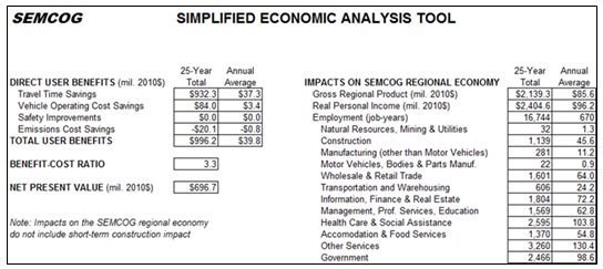
4.4.2. MINNESOTA DEPARTMENT OF TRANSPORTATION'S GUIDANCE ON BENEFIT COST ANALYSES FOR TRANSPORTATION PROJECTS
The Minnesota DOT has developed guidance, a spreadsheet template, and sample values that are used to streamline the performance of BCAs. The spreadsheet template serves to provide a standardized approach to planning and executing a BCA. The recommended values for some of the key analysis parameters ensure that different BCAs can be meaningfully compared to each other. The table below shows some of the recommended values from this guidance. The table below is shown as an example of how Minnesota is managing their BCA process, not as a recommendation that any agency should use specific values for any particular BCA. Note that the USDOT has provided guidance on the values that should be used in analyses to support applications for Federal TIGER grants in the TIGER Benefit-Cost Analysis (BCA) Resource Guide which is available on the web.51
| Variables | Current Value |
|---|---|
| Real Discount Rate | 2.20% |
| Auto-value of travel time savings per person-hour | $15.00 |
| Truck-value of travel time savings per person-hour | $27.20 |
| Auto-variable operating cost (dollars per mile) | $0.31 |
| Truck-variable operating cost (dollars per mile) | $0.95 |
| MnDOT Crash Values | Per crash |
| Fatal | $10,400,000 |
| Injury Type A | $540,000 |
| Injury Type B | $160,000 |
| Injury Type C | $80,000 |
| Property damage only | $3,300 |
| MnDOT = Minnesota Department of Transportation | |
4.4.3. RULES OF THUMB FOR ECONOMIC IMPACT ANALYSES
In Measuring the Economic Impacts of Projects and Programs, Glen and Burton Weisbrod provide the following rule of thumb for the magnitude of industry job and output multipliers for regions of different sizes:
Input/output models are available for county level or larger areas and provide multipliers that are estimates of local spending impacts assuming continuation of current inter-industry trade patterns and local flows of money into and out of the area. The magnitudes of these multipliers vary depending on the technology of the industry in which spending occurs and the size of the area economy –which affects the portion of these impacts that remain in the local economy and the portion that "leaks out" to outside areas. The multiplier values for most industries are generally around 2.5 - 3.5 for national impacts, 2.0 - 2.5 for State impacts and 1.5 - 2.0 for local area (large city) impacts.
4.4.4. TRANSPORTATION PROJECT IMPACT CASE STUDIES SYSTEM
The Transportation Project Impact Case Studies (T-PICS) System provides a way for practitioners to obtain case studies of economic impact analysis. This system, which is delivered through an interactive website, allows practitioners to enter data on the characteristics of their own project. They can then view projects that are similar to theirs, and use the data to estimate the likely impacts of their project. This approach allows the application of simplified rules of thumb based on economic impact analysis cases that are similar.
The tool works by drawing from a case study database of over 100 economic impact assessments to estimate the range of economic impacts likely to result from a specific type of project in a defined setting. "It provides a form of 'analysis by analogy' in that it identifies a reasonable range for expected impacts of proposed projects, based on prior experiences."52 It could serve as a screening tool for early stage project assessment.
4.4.5. SUPPLY CHAIN IMPACTS
Traditional analyses of freight transport investments is focused on estimating the travel time, vehicle operating cost, and other direct user benefits associated with freight transportation investments. Cost reductions that are experienced by carriers can be assumed to be passed on to shippers. These direct user cost reductions can then be fed into an economic model (such as Implan) and the economic (indirect and induced) impacts can be estimated. This approaches does not include the secondary logistics related benefits that will occur as businesses reorganize to take advantage of lower transportation costs. This reorganization might include substituting transportation for inventory or consolidating distribution centers. Leaving out these benefits can underestimate total benefits by as much as 10 to 40 percent. A simple rule of thumb that can be used is to assume that second order benefits will add approximatelt 15 percent to the total benefits of the project.53 54 Third order benefits can add an additional 0 to 10 percent in benefits, depending on the size of the transportation cost adjustment. This approach can provide an order of magnitude impact of the benefits, but provides little information on how this benefit might be distributed between industries. 55
| Infrastructure Benefit | Supply Chain Impact | Supply Chain Benefit Expressed as % of Operating Costs | Supply Chain Benefit Expressed as % of Transport Costs |
|---|---|---|---|
| 10% Transport Cost Reduction | Lower Material Cost by substituting cheaper sources | 0.10% | 1.50% |
| Consolidate Plants due to extended reach | 0.20% | 4.10% | |
| Switch modes and reduce shipment size, decreasing inventory | 0.10% | 1.20% | |
| 10% Capacity Increase | Less Safety stock | 0.10% | 1.10% |
| Rationalization of fleet and warehouse assets | 0.01% | 0.30% | |
| Secondary Effects | Increasing service levels | Not quantified | Not quantified |
| Converting cost savings into price reductions | Not quantified | Not quantified | |
| On-Demand supply chains | Not quantified | Not uantified | |
| Total Benefits as Expressed as % of Cost Component | n/a | 0.50% | 8.20% |
| Note: These benefits are indicative and preliminary estimates only that are based on average companies in a broad cross-section of industries, including many that have little transportation cost and don't move physical product. More precise estimates that are targeted at specific Supply Chain Types should be developed using the tools referenced throughout this text. Source: Boston Logistics Group, Inc. |
|||
12 The US government does not endorse any specific software or tools. [ Return to note 12. ]
13 This report is available at http://onlinepubs.trb.org/onlinepubs/ncfrp/ncfrp_rpt_008.pdf [ Return to note 13. ]
14 Cambridge Systematics and GeoStats LLP, NCFRP Report 8: Freight Demand Modeling to Support Public Sector Decision Making, National Cooperative Freight Research Program (Washington, DC: TRB 2010). Available at: http://www.trb.org/Main/Blurbs/164409.aspx [ Return to note 14. ]
15 Ibid. [ Return to note 15. ]
16 K. Kawamura, et al. Development of a Freight Policy Analysis Tool for Northeastern Illinois and the United States: Freight Activity Microsimulation Estimator. Urban Transportation Center (Chicago: University of Illinois at Chicago, December 2011). Available at: http://www.idot.illinois.gov/assets/uploads/files/transportation-system/reports/dpit/final%20report%20freight%20activity%20microsimulation%20estimator%20%28fame%29.pdf [ Return to note 16. ]
17 Federal Highway Administration, Report to Congress – 2013 Status of the Nation's Highways, Bridges, and Transit: Conditions & Performance, "Appendix A. Highway Investment Methodology – Valuation of Travel Time Savings." Available at: https://www.fhwa.dot.gov/policy/2013cpr/appendixa.htm#13 [ Return to note 17. ]
18 Federal Highway Administration, Freight Transportation Improvements and the Economy, FHWA-HOP-04-005 (Washington, DC: FHWA, 2004). Available at: https://ops.fhwa.dot.gov/freight/freight_analysis/improve_econ/ [ Return to note 18. ]
19 There are different approaches to measuring reliability including the 90th and 95th percentile travel time, travel time index, buffer index and the planning index. The 90th or 95th percentile travel time estimates how bad delay will be during the heaviest traffic days. "The travel time index is the ratio of a measured travel time during congestion to the time required to make the same trip at free-flow speeds. The buffer Index represents the extra buffer time (or time cushion) that most travelers add to their average travel time when planning trips to ensure on-time arrival. The planning time index represents the total travel time that should be planned when an adequate buffer time is included. The planning time index differs from the buffer index in that it includes typical delay as well as unexpected delay." [ Return to note 19. ]
20 Impact of Freight Delay to Economic Productivity. April 2014, http://tampabayfreight.com/wp-content/uploads/The-Impact-of-Freight-Delay-to-Economic-Productivity.pdf [ Return to note 20. ]
21 US Department of Transportation, TIGER Benefit-Cost Analysis Resource Guide (n.d.). Available at: http://www.dot.gov/sites/dot.gov/files/docs/TIGER%20BCA%20Resource%20Guide%202014.pdf [ Return to note 21. ]
22 Ibid. [ Return to note 22. ]
23 G. Giuliano, T. O'Brien, L. Dablanc, and K. Holliday, NCFRP Report 23 – Synthesis of Freight Research in Urban Transportation Planning, National Cooperative Freight Research Program (Washington, DC: TRB, 2013). Available at: http://onlinepubs.trb.org/onlinepubs/ncfrp/ncfrp_rpt_023.pdf [ Return to note 23. ]
24 MicroBENCOST may be ordered from the University of Florida, McTrans Center, http://mctrans.ce.ufl.edu/ [ Return to note 24. ]
25 British Columbia Ministry of Transport, MicroBENCOST Guidebook: Guidelines for the Benefit Cost Analysis of Highway Improvement Projects In British Columbia, 2014. Available at: http://www.th.gov.bc.ca/publications/planning/Guidelines/MBC-MASTER.pdf [ Return to note 25. ]
26 StratBenCost is distributed by McTrans. http://mctrans.ce.ufl.edu/ [ Return to note 26. ]
27 Federal Highway Administration, BCA.Net - Highway Project Benefit - Cost Analysis System User's Manual, April 2011. Available at: http://bca.decisiontek.com/docs/user.pdf [ Return to note 27. ]
28 Cambridge Systematics, NCFRP Report 12: Framework and Tools for Estimating Benefits of Specific Freight Network Investments, (Washington, DC: TRB, 2011). Available at: http://onlinepubs.trb.org/onlinepubs/ncfrp/ncfrp_rpt_012.pdf [ Return to note 28. ]
29 Caltrans, California Life-Cycle Benefit/Cost Analysis Model (Cal-B/C) User's Guide, February 2009. Available at: http://www.dot.ca.gov/hq/tpp/offices/eab/benefit_files/CalBC_User_Guide_v8.pdf [ Return to note 29. ]
30 Federal Highway Administration, Freight Benefit/Cost Study: Highway Freight Logistics Reorganization Benefits Estimation Tool Report and Documentation, FHWA-HOP-08-017 (Washington, DC: FHWA, 2008). Available at: https://ops.fhwa.dot.gov/freight/freight_analysis/econ_methods/bca_logistics/index.htm [ Return to note 30. ]
31 Economic Development Research Group, Inc. Development of Tools for Assessing Wider Economic Benefits of Transportation, Research Report S2-C11-RW-1, SHRP 2 Capacity Research Program (Washington, DC: TRB, 2014). Available at: http://onlinepubs.trb.org/onlinepubs/shrp2/SHRP2_S2-C11-RW-1.pdf [ Return to note 31. ]
32 Note that the benefits measured by this tool are the same ones that are measured by the Highway Freight Logistics Reorganization Benefits Estimation Tool discussed above. [ Return to note 32. ]
33 The REMI and TREDIS models are also based on input-output tables, and produce estimates of indirect and induced impacts. These models are discussed separately in the next section since they also utilize a more complex and dynamic modeling approach that also allows the user to estimate productivity impacts on the economy. [ Return to note 33. ]
34 Note that many EIAs may treat a project's construction cost as a stimulus and ignore the reality that the funds used to build the project may reduce government spending elsewhere or be taxed away from consumers and suppress spending by households in other areas of the economy. This can be accounted for by reducing expenditures from these other sectors. [ Return to note 34. ]
35 G. Weisbrod and B. Weisbrod, Measuring the Economic Impacts of Projects and Programs, (Boston: Economic Development Research Group, 1997). Available at: http://www.edrgroup.com/images/stories/Transportation/econ-impact-primer.pdf [ Return to note 35. ] ]
36 Brian B. Alstadt & Glen Weisbrod, "Unlocking the Potential of IMPLAN for Transport Impact Analysis," Presented at the 7th Biennial IMPLAN User's Conference, June 2008. [ Return to note 36. ]
37 Note that most economic models normally rely on the BEA input-output accounts, which allocate transportation costs among industries differently from the TSA. [ Return to note 37. ]
38 Bureau of Economic Analysis, "RIMS II Online Order and Delivery System" web page. Available at: https://www.bea.gov/regional/rims/rimsii/ [ Return to note 38. ]
39 https://www.bea.gov/regional/rims/rimsii/, page accessed June 4, 2015 [ Return to note 39. ]
40 Unlike EIA measures (e.g., output), productivity benefits (if measured accurately) would be additive to the value measured by BCA. [ Return to note 40. ]
41 TREDIS was also designed to be compatible with FHWA's highway benefit-cost guidelines and FAA's s aviation user benefit-cost guidelines. [ Return to note 41. ]
42 As discussed below, an organization that wants to use REMI to analyze the impacts of improvements in transportation system performance must utilize a pre-processor to format the input data. [ Return to note 42. ]
43 Total-factor productivity (TFP) is a variable which accounts for effects in total output not caused by traditionally measured inputs of labor and capital. If all inputs are accounted for, then total factor productivity (TFP) can be taken as a measure of an economy's long-term technological change or technological dynamism. TFP cannot be measured directly. Instead it is a residual, which accounts for effects in total output not caused by inputs. [ Return to note 43. ]
44 Michigan Department of Transportation, Economic Benefits of the Michigan Department of Transportation's FY 2010-2014 Highway Program, March 2010. Available at: https://www.michigan.gov/documents/mdot/MDOT_economicbenefitreport_202828_7.pdf [ Return to note 44. ]
45 Cambridge Systematics, "The Highway Economic Analysis Tool" web page. Available at: http://www.camsys.com/HEAT.htm [ Return to note 45. ]
46 John Kaliski and Glen Weisbrod, Guide to MCIBAS (Major Corridor Investment-Benefit Analysis System) and Its Economic Impact Analysis Component. April 10, 1998. Available at: http://www.edrgroup.com/pdf/mcibas-system-intro.pdf [ Return to note 46. ]
47 It may be the case that a state agency other than a DOT has obtained REMI Policy Insight without TranSight. Often, this would be the finance agency in a state government. It may be feasible for a state to obtain additional licenses for the DOT with the TranSight component included. Whether this would result in a cost for the DOT lower than that for getting the complete REMITranSight package separately would depend on the specifics of the existing arrangements between the state and REMI. [ Return to note 47. ]
48 For a lengthy and very detailed discussion of these two models, some readers might want to consult "Analyzing the Economic Impacts of Transportation Projects," published in September, 2013, by the Connecticut Academy of Science and Engineering. [ Return to note 48. ]
49 Freight & Economic Analysis Study. Talking Freight. November 14, 2012 [ Return to note 49. ]
50 SEMCOG, Southeast Michigan Freightand Economic Analysis, SEMCOG, July 2012. http://www.semcog.org/Portals/0/Documents/Plans-For-The-Region/Transportation/Freight/AppendixERelationshipBetweenFreightTransportationInfrastructureAndEconomicDevelopment.pdf [ Return to note 50. ]
51 USDOT, TIGER Benefit-Cost Analysis (BCA) Resource Guide. Available at: https://www.transportation.gov/sites/dot.gov/files/docs/TIGER%20BCA%20Resource%20Guide%202014.pdf [ Return to note 51. ]
52 Strategic Highway Research Program, "Transportation Project Impact Case Studies System" database. Available at: http://www.tpics.us/Default.aspx [ Return to note 52. ]
53 Cambridge Systematics, Inc., Economic Development Research Group, Inc., Boston Logistics Group, Inc., Guide to Quantifying the Economic Impacts of Federal Investments in Large-Scale Freight Transportation Projects. Prepared for Office of the Secretary of Transportation, U.S. Department of Transportation, August 2006. Available at: http://www.edrgroup.com/pdf/large-scale-freight-guide.pdf [ Return to note 53. ]
54 Note that these values are not in the U.S. DOT TIGER guidance, but rather are provided as approximations that have been discussed in the published literature. [ Return to note 54. ]
55 Cambridge Systematics, Inc., Economic Development Research Group, Inc., Boston Logistics Group, Inc., Guide to Quantifying the Economic Impacts of Federal Investments in Large-Scale Freight Transportation Projects. Prepared for Office of the Secretary of Transportation, U.S. Department of Transportation, August 2006. Available at: http://www.edrgroup.com/pdf/large-scale-freight-guide.pdf [ Return to note 55. ]