Cross-town Improvement Project Evaluation

2.0 Kansas City and Chicago C TIP Tests

2.1 Real-Time Traffic Monitoring

RTTM provides real-time predicted travel time information via the iPhone interface for primary and alternate routes, with route recommendations when warranted. Drivers can access this information pretrip by entering their origin and destination, after which the phone returns predicted travel times on the primary and alternate routes for that origin and destination pair. Drivers then select the route they want to take based on this information, with turn-by-turn directions provided by voice command from the iPhone.

During the trip, the iPhone sent GPS positional records to the C-TIP database, enabling the evaluation of driver compliance with recommended routes as well as comparison of actual to projected travel times for each trip (to assess travel time savings).

Route Compliance

The Real-Time Traffic Monitoring application was used by six drivers on five key intermodal lanes (origin-destination pairs) in Kansas City:

• BNSF to Topeka (Comtrak Logistics);
• Toyota to Grainger (Comtrak Logistics);
• UP to Toyota (Comtrak Logistics);
• BNSF to Musician’s Friend (IXT); and
• BNSF to NS (ITS).

Maps of primary and alternate routes for each lane are provided in Appendix A. Figure 2.1 shows driver compliance with the RTTM route recommendations at origin. This measures the degree to which drivers followed the RTTM route recommendations (whether or not RTTM recommended a default route or an alternate one). As the dashboard shows:

• Four of the five lanes had 100 percent compliance with RTTM route recommendations. This was the case with BNSF to Topeka, Toyota to Grainger, BNSF to Musician’s Friend, and BNSF to NS. However, on three routes (BNSF to NS, BNSF to Topeka, and UP to Toyota) RTTM never offered an alternate route, which implies that the primary route as defined in the application was always the best route from a travel time perspective. On the other lane (BNSF to Musician’s Friend), an alternate route was offered every time a driver made a travel time request at origin, and the driver proceeded to follow that route.
• The remaining lane (UP to Toyota) had zero percent compliance with the RTTM route guidance. However, this is owing to the fact that the true point of origin for these shipments was not the UP yard but a terminal consolidation point five miles away from the yard – a fact of which RTTM was not aware.

Figure 2.1 RTTM Route Compliance by Lane

Time Savings by Lane

Vantage dashboards also were developed to evaluate travel time performance on individual lanes. Figures 2.2 through 2.6 display travel time information by lane:

• BNSF to Topeka (Figure 2.2). There were 18 travel time requests on this lane, however RTTM never offered an alternate route. This is because the only alternate route defined in RTTM for this lane was a secondary road to the outskirts of Kansas City, which then reconnected with Interstate 70 to Topeka. During the test, however, there was never enough congestion on I-70 to make the alternate route faster. In fact, none of the trucks on this route actually went all the way to Topeka – they all stopped at points between the BNSF terminal and Topeka instead. Therefore, it is not possible to evaluate travel time savings or the accuracy of the RTTM projections.
• Toyota to Grainger (Figure 2.3). There were five travel time requests on this lane, all of which yielded an alternate route recommended by RTTM. Trucks took the alternate route on all five of these occasions. However, the primary and alternate projected travel times are the same (26 minutes). In any event, none of the trucks that requested travel times on this lane sent positional data. This could be due to several factors, including drivers turning off the iPhone after requesting travel time, or drivers and other fleet staff “testing” the app to learn about its functionality.
• UP to Toyota (Figure 2.4). There were five requests for travel time during the test period on this lane but RTTM never offered an alternate route here either. As noted above there was zero compliance with RTTM recommendations on this route because the actual origination point was not the same as the one assumed by RTTM. The average primary route projected travel time was 33 minutes, but it is not possible to evaluate this against actual travel times because of this routing issue.
• BNSF to Musician’s Friend (Figure 2.5). RTTM received 17 requests for travel time information on this lane, for which the system recommended an alternate route all 17 times. Moreover, the drivers actually followed this alternate route 100 percent of the time. On average, RTTM predicted the primary route travel time to be 31 minutes and the alternate route to be 24 minutes. Actual travel time varied from projected by an average of five minutes, and actual times were within 10 percent of projected times 22 percent of the time.
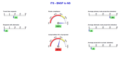
• BNSF to NS (Figure 2.6). There were nine travel time requests on this lane, but RTTM never offered an alternate route. Route compliance was 100 percent since drivers always took the default route which also was recommended by RTTM. Travel time accuracy was fairly good on this lane, with an average variance of three minutes between projected and actual travel times. Actual travel times were therefore within 10 percent of projected times 57 percent of the time.

Figure 2.2 RTTM Travel Time Performance, BNSF to Topeka

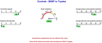
Figure 2.3 RTTM Travel Time Performance, Toyota to Grainger

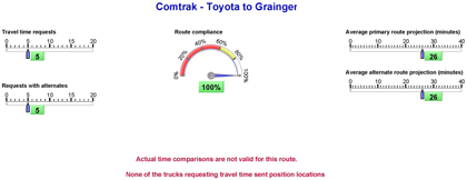
Figure 2.4 RTTM Travel Time Performance, UP to Toyota

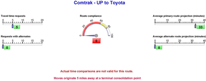
Figure 2.5 RTTM Travel Time Performance, BNSF to Musician’s Friend

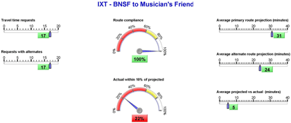
Figure 2.6 RTTM Travel Time Performance, BNSF to NS

Emissions Reduction

Diesel emissions are a function of distance traveled and speed. Therefore, if a route recommended by RTTM is shorter in distance than the default route, there could be an emissions reduction associated with it. The evaluation team therefore used common emissions factors to convert RTTM distance and delay savings to reduction in diesel emissions.

RTTM was able to achieve modest reductions in greenhouse gas and criteria pollutant emissions during the Kansas City test period. (Criteria pollutants are six common air pollutants for which EPA sets National Ambient Air Quality Standards following requirements of the Clean Air Act.) For this evaluation, CS estimated the emissions reductions that would be achieved for five EPA-designated criteria pollutants, including carbon monoxide, oxides of nitrogen, volatile organic compounds, and diesel particulate matter. Particulate matter is broken down into two categories: PM₁₀ (particles less than 10 microns but more than 2.5 microns in diameter) and PM_2.5 (particles less than 2.5 microns in diameter). Reductions in greenhouse gas emissions (measured in carbon dioxide equivalents, or CO₂eq) also were estimated.

Emissions factors in grams per mile specific to short-haul combination trucks in the four-county Kansas City area were obtained from the EPA MOVES model (see Table 2.1). Factors are divided into speed bins from 2.5 mph to 75 mph.

Table 2.1 EPA MOVES Dray Truck Emissions Factors, In Grams per Mile

Speed (MPH)	Carbon Monoxide (CO)	Oxides of Nitrogen (NOx)	Volatile Organic Compounds (VOC)	Carbon Dioxide Equivalents (CO2eq)	Particulate Matter (PM10)	Fine Particulates (PM2.5)
2.5	21.99685	54.16616	6.041066	9651.828	3.337922	3.237911
5	10.99843	27.08309	3.020535	4825.908	1.66896	1.618954
10	6.336506	16.69532	1.56982	3097.472	1.071154	1.039059
15	4.99147	14.53054	1.080162	2830.331	1.019193	0.988655
20	4.153309	13.09162	0.825059	2576.837	0.94696	0.918586
25	3.735008	12.00771	0.697809	2402.457	0.888957	0.862322
30	3.403155	11.7275	0.608871	2362.748	0.859345	0.833596
35	2.955478	10.14686	0.553779	1982.124	0.646784	0.627405
40	2.755327	9.910763	0.510617	1943.435	0.604152	0.586051
45	2.599646	9.727128	0.477047	1913.348	0.570996	0.553888
50	2.439501	9.416561	0.449968	1825.176	0.499143	0.484189
55	2.29002	9.073868	0.427016	1719.147	0.415935	0.403474
60	2.191812	8.968768	0.404485	1690.702	0.379639	0.368266
65	2.124675	9.477438	0.383504	1802.04	0.396157	0.38429
70	2.067133	9.913411	0.36552	1897.47	0.410317	0.398025
75	1.959225	9.605677	0.344137	1842.103	0.396435	0.38456

Source: EPA MOVES model. Note that these factors use national default MOVES input data and are not allowed to be used for SIPs or conformity analysis.

Emissions benefits were calculated using the average projected speed in miles per hour (based on projected travel time and known distance) for the longer and shorter routes in each lane. Emissions factors for the appropriate speed bin were then taken from Table 2.1 and used to calculate expected emissions for each pollutant on the primary and alternate route. The difference between these two calculations is the estimated emissions reduction associated with C-TIP RTTM.

It is only possible to evaluate emissions reductions on two cross-town lanes since alternate routes were not offered on the other three. Figure 2.7 highlights the results for the two lanes that could be evaluated:

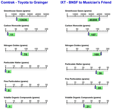
• On the Toyota to Grainger route, RTTM is estimated to have reduced greenhouse gas emissions by about 13,600 grams of CO₂ equivalents (CO2eq). Carbon monoxide was reduced by 11 grams; nitrogen oxide by 78 grams; and VOCs by 1 gram. There was no measurable improvement in particulate matter emissions.
• On the BNSF to Musician’s Friend route, RTTM reduced GHG emissions by about 40,000 grams. Carbon monoxide was reduced by 107 grams; oxides of nitrogen by 168 grams; PM₁₀ by 36 grams; PM_2.5 by 35 grams; and VOCs by 21 grams.

Although these reductions are rather modest due to the relatively small number of trucks involved in the test, emissions benefits would presumably be greater if the system were deployed more widely, especially in a larger intermodal market like Chicago. This would help mitigate some of the known public health problems associated with goods movement. For instance, nitrogen oxide (NOx) is a precursor to ozone, which has been linked to respiratory problems, skin irritation, asthma, and other ailments. Particulate matter has been linked to heart disease and cancer. Diesel engines are significant sources of both NO_x and PM pollution. (Federal Highway Administration, Freight and Air Quality Handbook, May 2010.) Reductions in greenhouse gases, meanwhile, help mitigate global climate change.

Figure 2.7 RTTM Emissions Reduction

2.2 Dynamic Route Guidance

Dynamic Route Guidance (DRG) provides truckers with real-time travel time information for key cross-town intermodal routes and can reroute them around congestion through in-cab voice commands, thus eliminating potential driver distraction issues. In the Kansas City test, redirections could occur whenever trucks approached a predefined “decision point” along a given lane. Prior to reaching the decision point, DRG would recalculate the predicted travel time based on current information; if it found a delay ahead (due to a traffic accident or similar event), it would verbally instruct the driver to take the alternate route with turn-by-turn directions. Whenever DRG redirected a truck, the GPS positional data was used to assess whether the driver followed the redirection and also to compare the projected travel time on the original route from the decision point to the actual travel time on the diverted route, also from the decision point.

During the test period, there were 95 total trips with DRG route guidance on the five Kansas City intermodal lanes, of which 30 were redirected to avoid congestion. DRG provided en-route redirections on three lanes:

• Toyota to Grainger (Comtrak Logistics);
• UP to Toyota (Comtrak Logistics); and
• BNSF to Musician’s Friend (IXT).

Maps showing the DRG redirects on each of these three routes are provided in Appendix A. There were no redirects on the BNSF to NS and BNSF to Topeka routes during the test period.

Route Compliance and Time Savings

Figures 2.8 to 2.12 show the route compliance and time savings results of the DRG test.

• Toyota to Grainger (Figure 2.8). There were 13 en-route redirects on this lane during the test period out of 18 total trips. Drivers followed the recommended reroute 77 percent of the time. DRG recommended a reroute essentially at the outset of these trips (zero minutes from origin until change). The average projected travel time on these redirects was 27 minutes, saving drivers an average of five minutes. Actual travel times were at variance with projected ones by an average of three minutes, and the DRG projected time at the decision point was within 10 percent of the actual time on half of these trips.
• UP to Toyota (Figure 2.9). There were 29 total DRG trips on this lane. Of these, there were 11 redirects, all of which the drivers followed. The average time from trip origin to DRG redirect was six minutes, and the average projected travel time on the reroutes was 16 minutes from the decision point. These reroutes saved drivers six minutes of travel time on average, but the average difference between predicted time and actual time also was six minutes – leading to low travel time accuracy on this lane since the trips were so short.
• BNSF to Musician’s Friend (Figure 2.10). There were six DRG redirects on this lane during the test period (out of a total of 19 trips), and drivers followed the redirection 83 percent of the time. DRG recommended a reroute, on average, just two minutes into the trip. The average projected travel time for the reroutes was 23 minutes. The DRG redirection saved drivers seven minutes of travel time on average. In terms of travel time accuracy, the average variance between actual and projected travel time was four minutes, and DRG projected travel time was within 10 percent of the actual travel time for about two-thirds of the trips during the test.
• BNSF to Topeka (Figure 2.11). There were 20 total trips on this lane; however DRG never redirected drivers to an alternate route, so it is not possible to measure DRG travel time projections or time savings on this route.
• BNSF to NS (Figure 2.12). There were nine trips on this route during the test period but no DRG redirects, so it is not possible to measure DRG benefits on this route either.

Figure 2.8 DRG Performance, Toyota to Grainger

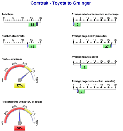
Figure 2.9 DRG Performance, UP to Toyota

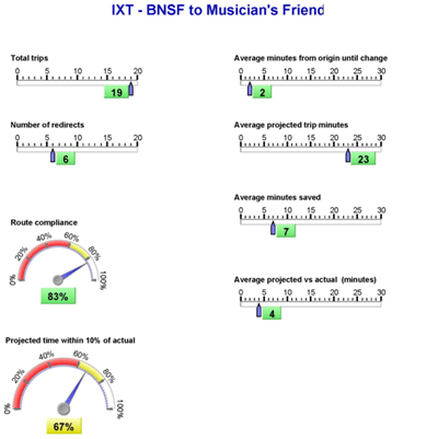
Figure 2.10 DRG Performance, BNSF to Musician’s Friend

Figure 2.11 DRG Performance, BNSF to Topeka

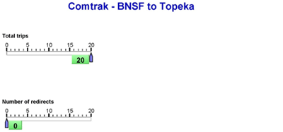
Figure 2.12 DRG Performance, BNSF to NS

Emissions Reduction

DRG emissions reductions also were assessed on these three cross-town lanes. The calculations were performed the same way as for RTTM, except the speed and distance calculations were determined from the point of redirection for each route rather than the point of origin. The same EPA emissions factors shown in Table 2.1 were used to assess DRG emissions savings. Figure 2.13 presents the estimated emissions reductions by lane.

• On the Toyota to Grainger lane, DRG is estimated to have reduced total GHG emissions by more than 35,000 grams, nitrogen oxides by 202 grams, and carbon monoxide by 28 grams during the test period. There was no reduction in particulate matter, and reductions in volatile organic compounds were negligible.
• For the BNSF to Musician’s Friend lane, GHG emissions were reduced by about 14,000 grams. NO_x was reduced by 59 grams, while CO was reduced by 38 grams. Other pollutants had more modest reductions, including 13 grams of PM₁₀; 12 grams of PM_2.5; and seven grams of VOCs.
• The UP to Toyota lane had the greatest emissions reductions under DRG. GHGs on this lane were reduced by nearly 60,000 grams of CO₂eq. Nitrogen oxides fell by 271 grams and carbon monoxide by 89 grams. PM₁₀ and PM_2.5 were reduced by 28 grams and 27 grams, respectively, while VOC emissions fell by 16 grams.

Overall these savings are modest but not unexpected given the scale of the deployment. The test did show, however, that there is scope for emissions reduction through freight dynamic mobility applications.

Figure 2.13 DRG Emissions Reduction

2.3 IMEX Analysis

IMEX is a collaborative on-line dispatch model designed to facilitate information exchange between intermodal rail terminals and the dray trucking community, with the goal of reducing unproductive moves to the greatest extent possible. Using data feeds from trucking firms and railroads, IMEX produces a daily work plan that optimizes container and chassis moves between cross-town railroads. The work plan is designed to accomplish the necessary moves with the fewest possible bobtail trips. IMEX proposes a carrier for each cross-town (either ITS or Greer). Railroads can view this plan and assign work orders accordingly, as shown in Figure 2.14.

Figure 2.14 IMEX Trip Assignments

Source: SAIC.

Due to several external factors, including a decline in freight volumes brought about by the recession and the retirement of a key C-TIP champion at a Class I railroad, Kansas City railroads did not participate in the C-TIP operational test. This made it impossible to evaluate the actual benefits of C-TIP IMEX since the railroads did not use the system. Therefore, the evaluation team instead conducted a simulation test to estimate the potential benefits of IMEX.

Kansas City

The Kansas City IMEX simulation test, conducted from October 1, 2010 to January 31, 2011, provided a total of 1,663 cross-town drayage moves for analysis. These moves included cross-town transfers between the Union Pacific Neff Yard and the Norfolk Southern Voltz Yard, and between the BNSF Argentine Yard and NS Voltz Yard. The railroads provided gate move data, including the date and time a container was unloaded; the origin and destination terminals; and a container ID number.

Figure 2.15 provides a summary of terminal move activity during the Kansas City test period and IMEX matched moves. The vast majority of moves originated at either the BNSF Argentine or UP Neff yards. This is because the prevailing traffic pattern for cross-towns in Kansas City is from western railroads (e.g., BNSF or UP) to eastern railroads (e.g., NS). The BNSF and UP railheads accounted for 1,588 of the cross-towns in the test period, or 95 percent of the total. The total number of matches averaged about 30 per month except for November when it rose to 71 matches.

Of the 1,663 moves, IMEX identified 163 potential “matches,” or containers that could be sequentially matched and moved by the same driver, thus eliminating a bobtail. A potential match in IMEX occurred whenever the same terminal had a container destined to it and also had a container move originating from it. In that event, the same driver could theoretically bring the first container to the terminal, drop it off, and load up the next container without making a bobtail move. For purposes of distributing matched loads, it was assumed that each driver could handle five containers per day. However, in practice there were never enough matches in one day to require more than one driver.

Figure 2.15 C-TIP IMEX Terminal Move Summary, Kansas City

It is important to note that not all IMEX matches correspond to actual matches. Of the 163 matches identified by IMEX, only 28 could be verified as cross-town moves that were performed in sequence by the same driver. Railroads and dray carriers did not always match loads for a variety of reasons:

• The IMEX dispatch model assumed that boxes can sit all day in a terminal if necessary in order to be matched; however, in practice this is rarely the case as railroads typically want grounded containers out of their yards as soon as possible.
• Draymen in Kansas City do not plan their entire day far enough in advance to take advantage of matching opportunities, and in any event the railroads typically don’t give dray carriers notice until a unit is on the ground anyway – all of which makes it hard to coordinate moves across the space of many hours.
• Overall, truckers may view it as too much trouble to pick up a matched load when doing so would only save them about 15 minutes (at least in the Kansas City context). In Kansas City, the rail terminals are close enough together to allow a trucker to drop off a box, bobtail back to the originating terminal, and deliver another box within one hour – thus minimizing the potential time savings associated with picking up a matched load.

Additionally, overall volumes and traffic patterns changed dramatically just prior to the test period due to the recession and changing railroad operational strategies, leading to drastically reduced load matching during the C-TIP deployment phase. These cumulative factors contributed to low overall participation in the program amongst railroads and dray carriers.

Nonetheless, this initial IMEX deployment did prove the concept that a specially designed technology could address the known inefficiencies associated with cross-town rubber tire interchanges between railroads. It is possible that greater benefits could be achieved in a larger rail market such as Chicago.

Figure 2.16 is another Vantage dashboard describing key C-TIP IMEX performance metrics. The top row of gauges shows total moves, total C-TIP matches, and actual matched moves. The bottom set of gauges describe the potential empty trips/miles eliminated and fuel saved if all stakeholders had followed the IMEX work plan during the test period. Empty mileage and fuel savings were calculated using the following assumptions:

• Distance between terminals is eight miles (UP Neff to NS Voltz; there were no matches from the NS back to the BNSF during the test); and
• Dray truck fuel economy averages six miles per gallon (a commonly accepted value in the trucking community).

The number of empty miles saved is thus the distance between the terminals multiplied by 135 trips. Fuel savings are then derived by dividing average fuel economy into total miles saved.

Figure 2.16 C-TIP IMEX Performance Metrics, Kansas City

Using these assumptions, if C-TIP had been fully utilized during the period, it would have eliminated 135 empty truck trips (163 C-TIP matches minus 28 actual matches). This would have eliminated 1,080 empty miles and saved 180 gallons of diesel fuel.

These potential mileage and fuel savings also would lead to emissions reductions. CS estimated the potential IMEX emissions reductions using the same EPA emissions factors used in the RTTM/DRG analysis. For analytical purposes, it was assumed that trucks traveling between the two terminals would average 30 mph. (Google Maps reports a travel time of 18 minutes between the two points, which is about 27 mph.) Therefore, emissions factors for the 30 mph speed bin were chosen from Table 2.1 for the analysis.

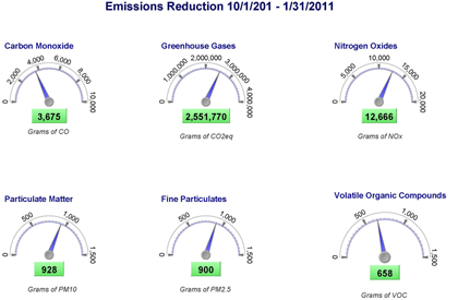
The results are provided in Figure 2.17. As the Vantage dashboard shows, given this set of assumptions, C-TIP IMEX would have reduced carbon monoxide emissions by 3,675 grams, greenhouse gases by about 2.5 million grams of CO₂eq, oxides of nitrogen by 12,666 grams, PM₁₀ by 928 grams, PM_2.5 by 900 grams, and VOC by 658 grams.

Figure 2.17 C-TIP IMEX Potential Emissions Reduction, Kansas City

Chicago Terminal

A similar ‘what if’ analysis was conducted for intermodal transfers in Chicago, which is by far the nation’s largest rail hub. The Chicago test relied on gate move data provided by the UP and CSX railroads. The data includes 9,890 intermodal moves between these two railroads in Chicago, made between January 1, 2011 and April 30, 2011. These moves involved four UP terminals and two CSX terminals in the Chicagoland region. These data were loaded into IMEX, which then provided a daily optimal work plan as in Kansas City. The work plan used the same logic as the Kansas City test, except that the gate move data were analyzed in one batch rather than on a daily basis since four months’ worth of data were received all at once.

The following assumptions were used:

• The average dray distance between terminals is 25 miles;
• The cutoff for cross-town deliveries is 5:00 p.m. each day; and
• Dray truck fuel economy averages 6 mpg.

Results were stratified into 24-hour, 12-hour, 3-hour, and 15-minute ‘windows’, where each time window represents the total time available to make the cross-town delivery from container de-ramping at the originating terminal to the 5:00 p.m. cutoff at the receiving terminal.

Figure 2.18 shows theoretical C-TIP IMEX performance for the Chicago terminal under these assumptions. Clearly, the potential is much greater in a large intermodal market like Chicago. Under the 24-hour window, there are nearly 2,000 matches; if all of these matches actually occurred it would save more than 49,000 empty truck miles and about 8,200 gallons of diesel fuel. Interestingly, under a 12-hour delivery window the potential matches, miles saved, and fuel saved do not decrease that much. Even under the 3-hour window, the system finds more than 1,600 matches which would save 41,000 empty miles and cut fuel use by nearly 7,000 gallons. This suggests that substantial benefits could be realized even under real-world operational constraints such as tight cutoff times for cross-town freight.

Figure 2.18 C-TIP IMEX Performance, Chicago Terminal

As in Kansas City, these fuel savings also would generate significant reductions in key pollutants and greenhouse gases. For the analysis of emissions savings, CS used the following emissions factors:

• CO: 3 grams per mile;
• CO₂eq: 2,000 grams per mile;
• NO_x: 11 grams per mile;
• PM₁₀: 8 grams per mile;
• PM_2.5: 0.75 grams per mile; and
• VOC: 0.6 grams per mile.

These factors were adapted from the Kansas City emissions factors and represent values in between the 30 mph and 35 mph speed bins. As shown in Figure 2.19, the potential emissions reduction is substantial due to the volume of cross-town traffic in Chicago. Assuming the originating railroad had 24 hours to cross-town a container, IMEX could potentially reduce particulate matter emissions by over 63,000 grams; other criteria pollutants (NO_x, VOC, and CO) by nearly 700,000 grams; and greenhouse gas equivalents by almost 100,000 grams. Savings under the 12-hour window are similar in size. Assuming that the 3-hour window is the most realistic, the reductions are still substantial, totaling 53,000 grams of particulate matter, 567,000 grams of other criteria pollutants, and 82,000 grams of CO₂ equivalents. Combining all criteria pollutants (PM plus other criteria pollutants), IMEX could potentially have eliminated more than six-tenths of a ton of harmful diesel emissions in Chicago during the four-month test period. If all six Class I railroads that operate in Chicago participated fully in IMEX, the savings would likely be much greater.

Figure 2.19 C-TIP Potential Emissions Reduction, Chicago Terminal

2.4 C-TIP User Interviews

Interviews with C-TIP system users were conducted to better assess non-quantitative aspects of the application. CS contacted drivers who were using the RTTM/DRG application on iPhones in their cabs as well as dispatchers/terminal managers who were involved in the test. Separate questionnaires were developed for truck drivers and terminal managers/dispatchers. The interview instruments are provided in Appendix B. Responses were collected from two drivers, one dispatcher, and one terminal manager. Feedback is somewhat limited due to the small number of users and difficulties with engaging truck drivers who are not often in an office where they may be reached by telephone. However, the responses that were gathered offer some useful insights about the initial C-TIP deployment, which are summarized below.

• In general, users liked the idea of having a smart phone application that provided routing information, but they did note some practical obstacles to the RTTM/DRG app. Two users from ITS noted that the phone never recommended alternate routes, even during construction on the primary route which caused significant delays. There also were concerns about the truck-friendliness of alternate routes. Even so, most felt the application was convenient to have and could be beneficial.
• Some interviewees felt the user interface could be improved, mainly by reducing the number of steps required to obtain a route. One driver had unspecified problems with the touch screen interface. Older drivers who may not have been highly ‘tech-savvy’, as well as those for whom English was a second language, required additional training to use the app. However, once they got used to it things seemed to run fairly smoothly.
• One driver did report an example of a significant time savings achieved with DRG. This driver reported that a wreck on I-35 caused the phone to reroute him around the incident, which saved him about five minutes in travel time on that particular trip. The same driver also noted that the application was effective at increasing the number of turns he could make in a day.
• In terms of improvements to the information provided, in general the interviewees didn’t see much value in providing estimates of the amount of fuel they could save by taking an alternate route. The terminal manager and one of the drivers indicated that drivers tend to monitor their fuel use closely already. The other driver – who actually did receive alternate routings – stated that his fuel use was about the same and the main benefit was really productivity. Some interviewees felt that an automatic load notification system would be useful (i.e., if the system alerted drivers when a container was released for pickup), but it would still have to keep the dispatcher in the loop to avoid multiple drivers converging on one spot to get a load.

previous | next