Traffic Analysis Toolbox Volume XII:
Work Zone Traffic Analysis – Applications and Decision Framework
Chapter 5. Establishing an MOTAA Decision Framework
This chapter will provide guidance on developing and applying an Maintenance of Traffic Alternatives Analysis (MOTAA) decision framework. The chapter is organized as follows:
- The first section will provide an overview of the decision-making process within a work zone MOTAA. It also will describe the factors that shape the decision-making process, as well as the traditional decision-making frameworks often applied in work zone traffic analysis.
- The second section will highlight several analysis methodologies that can aid in the prioritization of criteria, and factors and/or thresholds used to evaluate and compare work zone alternatives.
- The third section will present evaluation methodologies that aid decision-makers in identifying the optimum alternative or combination of strategies that will best fit the project.
- The fourth section will highlight several decision-making tools that help automate the analysis needed to choose among different work zone alternatives.
5.1 Overview of an MOTAA Decision Framework
The Decision Framework within an MOTAA Process
The MOTAA decision-making methods and evaluation framework are typically applied after the agency has developed their set of potential work zone alternatives. The alternatives are generated during the planning process after the agency has established its set of goals and objectives. The list of alternatives is further refined once the agency has narrowed down the alternatives to only those feasible, either through a fatal flaw or other type of analysis. The decision-making process then occurs after the agency has evaluated the performance of the project, along with their potential alternatives using a selected analysis tool. After the modeling analysis, a set of performance measures and other factors, such as those described in Chapter 6, will be used to form the criteria that determine how well the alternative meets the goals and objectives of the project. How these criteria or measures are used in determining the recommended alternative will be a function of the selected decision framework.
Traditional Decision-Making Framework
While no standardized decision-making framework has been established in a typical MOTAA process, the most common decision-framework used to date typically follows rule-based reasoning. Rule-based reasoning uses “if-then-else” rule statements. For instance, in an MOTAA process, an “if” statement may evaluate whether an alternative meets a particular criterion. If the alternative does meet the criterion, the “then” statement may indicate that the alternative should be chosen. If the alternative does not meet the criterion, the “else” statement may specify to reject the alternative, suggest revising the alternative or choose the alternative with the least impact. An example of a typical rule-based reasoning for a hypothetical work zone scenario is illustrated in Figure 17.
Figure 17. Example of a Traditional Decision-Framework
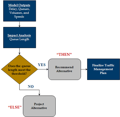
The traditional MOTAA decision-making process begins with the formulation of work zone alternatives – the development of different work zone configurations and strategies. Afterwards, these alternatives are analyzed based on performance measures or standards set by the agency. If the alternatives do not meet the standards, they will either be revised or replaced by other alternatives that comply with the set performance measures. The alternative that best meets the standard(s) or has the least negative impacts is selected.
Decision Methodologies
In the typical decision frameworks, the decision criterion used is often dependent upon one type of measure – a mobility, safety, or cost measure. While this method may address one of the objectives of the project, it does not account for a multidimensional way of comparing alternatives. The methodologies discussed in this section present additional analysis methods and tools that account for how multiple factors can form a criteria for evaluating and choosing among alternatives. The following decision-making frameworks serve as potential options for an agency to consider. However, in some cases, an agency may be required to follow a standard approach established by their organization.
In these types of decision-making frameworks, there are often two levels of analysis. The first level typically applies factor prioritization analysis methods. These analysis methods can prioritize and/or assign weights to the factors that are used to compare and evaluate potential work zone alternatives. The second level of analysis typically employs scoring and/or evaluation matrices for recommending an alternative(s). These methodologies provide the structure for the decision framework. They determine how the prioritized and/or weighted criterion determined in the factor prioritization procedures can be used to evaluate and choose among the alternatives.
Below is an overview of the factor prioritization methodologies featured in this chapter. Further information, including example work zone applications of such methodologies, is provided in Section 5.2.
- Delphi Method – This method offers a methodology for identifying and prioritizing factors or criteria through surveying a panel of experts, who then works towards reaching a consensus on the priority of the factors based on their level of importance to the project.
- Factor Analysis – This analysis is a general scientific method for analyzing data by uncovering order, patterns, and regularity in the data. (Rummel, R.J. Applied Factor Analysis. Northwestern University Press, Evanston, Illinois, 1970.) The overview focuses on its use for prioritizing and weighting criteria.
- Ranking Analysis – The ranking method calculates normalized criteria weights based on how a panel of surveyed or polled participants ranks the factors based on their level of importance.
- Ratio Analysis – The analysis calculates normalized criteria weights based on surveyed participants’ responses on how criteria elements measure up against each other.
- Paired Comparison Analysis – In a paired comparison analysis, criteria are compared against each other one pair at a time. A criterion’s score or weight is based on the number of times it is preferred over others.
- 100-Point Distribution – In a 100-point distribution, criteria weights are decided based on how an individual or group distributes 100 points amongst the factors/criteria.
An overview of the work zone alternatives evaluation frameworks featured in this chapter are listed below. The factor prioritization methodologies previously identified are often incorporated within these evaluation frameworks to guide how the factors or criteria are used in recommending an alternative(s). Further information on how to apply these methodologies within an MOTAA decision framework is provided in Section 5.3.
- Multi-Criteria Decision-Making Models (MCDM) – Mathematical methodologies that evaluate and compare the utility or relevancy of alternatives to the project goals and objectives. There are two MCDM techniques: Simple Additive Weighting (SAW) and Analytical Hierarchy
- Process (AHP), which are featured in this chapter.
- Kepner Tregoe (KT) Method – Decision-making that features a step-by-step approach, evaluating each alternative by its impacts, risks, and opportunities.
- Benefit/Cost Analysis – This compares the sum of all costs with the sum of all benefits associated with an alternative. The benefit/cost ratio can be used to compare alternatives.
Choosing a Decision-Making Framework
There are several general considerations an agency should consider in determining the framework or analysis method best suited for choosing among different work zone alternatives. Sections 5.2 and 5.3 discuss these considerations in further details, as well as addressing many of the methodologies’ limitations and strengths. Some of these considerations include the following:
- Level of Data Collection Effort – Several of the methodologies may require gathering data from case studies, extracting performance measures from the analysis tools, or polling/surveying people in order to develop the criteria for choosing amongst alternatives. The agency needs to be aware of the data collection effort needed to conduct a particular decision-making methodology.
- The Complexity of the Analysis – The analysis methodology may range from simple to more complex mathematical models. The agency must take into consideration whether or not they have the appropriate tools or expertise to perform a particular decision-making methodology.
- Time – Some of the methods are more time-consuming than others. An agency should choose the methodology that best fits their time line.
- Project Complexity – The complexity of the project may impact which methodology is best suited for the agency. Since some methodologies may be more resource intensive than others, it may not make sense to use highly complex decision-making frameworks for simple, short-term projects.
5.2 Approaches to Factor Prioritization
This section provides further detail on the use of the factor prioritization methodologies for an MOTAA application. As previously mentioned, analysis methods can aid agencies in prioritizing their selected factors by level of importance to the project, as well as in creating weighted criteria. The weighted factors can then be integrated into a weighting/scoring method to choose among alternatives.
At this stage in the process, the agency should have a list of factors, both quantitative and qualitative, that have relevancy to the project characteristics, goals, and objectives. These factors should indicate how well the alternative can meet the goals and objectives established by the agency for the work zone project. Some example criteria include level of delay at the work zone, average speeds, accident rates, and the work zone alternative’s impacts to operating and maintenance costs.
Various methodologies are described below and each is structured to contain the following:
- An overview of the approach;
- Pros and cons of the methodology; and
- An example application.
A summary table (Table 37) highlights the particular features and capabilities of these methodologies, their strengths, and weaknesses.
Table 37. Factor Prioritization Methodologies Summary
| Methods/Considerations |
Project Complexity Suited For |
Analysis Complexity |
Level of Data Needs |
Development Time |
Analysis Time |
Potential for Bias/Conflict |
| Delphi |
Medium-High |
Medium |
High |
High |
High |
Medium |
| Factor Analysis |
Medium-High |
High |
High |
Medium |
Medium |
Low |
| Ranking |
Low-Medium |
Low |
Medium |
Medium |
Low |
Medium |
| Ratio |
Low-Medium |
Low |
Medium |
Medium |
Low |
Medium |
| Paired Comparison Analysis |
Low |
Low |
Medium |
Low |
Low |
High |
| 100-Point Distribution |
Low |
Low |
Low |
Low |
Low |
High |
Delphi Method
Approach Overview
The Delphi Method offers a methodology for identifying the factors or criteria that can be used to screen alternatives. The steps for applying the Delphi Method are:
- Step 1 – The careful selection of panel experts from disciplines most relevant to the project and its goals and objectives.
- Step 2 – Distribute questionnaires that will narrow down the attributes, and determine the level of importance and average utility values of each of the attributes. A factor prioritization method can be used to determine the level of significance of each attribute using the survey results.
- Step 3 – Repeat Step 2 as necessary.
- Step 4 – After all rounds of the questionnaire have been completed, the end result is a set of weighted attributes to be used in ranking the alternatives.
The duration of this approach, including the number of questionnaire rounds and the number of experts comprising the panel, is dependent on available resources and other project characteristics. Table 38 lists some general pros and cons of the Delphi Method.
Table 38. Pros and Cons of the Delphi Method
| Pros |
Cons |
- Finds consensus among differing opinions
- Less biased
- Allows participants to be anonymous
- Well selected expert panel can provide broad analytical perspectives on impacts
- Flexibility and applicability to various issues
|
- Judgments are still made by a select group and not necessarily representative
- Technique can be time-consuming
|
Example Application
The following presents a hypothetical case study for the application of the Delphi Method in MOTAA. For ease of presentation of this technique, the example focuses on the analysis of two broad project goals – improvement of standard construction strategies/methodologies and minimizing traffic, environmental, and economic impacts.
The agency in this case has developed potential alternatives. Additionally, they have developed a list of potential factors, labeled “objectives” that can be used to screen the alternatives. In order to determine which factors have the most significance to the project goals, the agency applies the Delphi Method (see Table 39 for Delphi structure) through the following steps:
- Step 1 – The agency assembles an expert panel. The panel participants in this case should have experience in work zone management, traffic management, and/or work zone relevant research and have an understanding of the agency’s goals.
- Step 2 – The agency assembles the first round of three questionnaires. This first round asks the panel to list five objectives that are of relevance to the project and its goals. After the results from the first round are turned in, the evaluator(s) can choose to reduce the list in preparation for the next round.
- Step 3 – In the second round of questionnaires, the panel is asked to rank the refined list of objectives by desirability and importance to the project. Table 40 lists the reference scale and definitions for desirability and importance. In this example, the higher the value, the more desirable or important the objective is to the project. After the panel responses for the second round have been turned in, the evaluator(s) can then average the group scores for both desirability and importance. Table 41 shows example results.
- Step 4 – The evaluator determines a threshold for narrowing down the list of objectives. In this example, objectives that scored lower than 3.0 for either importance or desirability was eliminated for the next round. Objective that are bold in Table 41 were eliminated in the third round.
- Step 5 – For the third round, the evaluator revises the motivations for the questionnaire. The panel participants are again asked to rank the objectives by level of desirability and importance. However, in this round they rank the objectives according to specified categories such as project management, safety, mobility, and environmental impacts as shown in Table 42.
- Step 6 – After the responses from the third round have been collected, the evaluator can then create a weighting scale based on the results. In Table 42, the evaluator determined the weights by calculating the objective’s score as a percentage of the total score for that category.
Table 39. Delphi Technique Example
| Goals: Improve standard construction strategies and methodologies; minimize traffic, environmental, and economic impacts |
 |
Round 1 – Generating List of Objectives |
Round 2 – Desirability and Importance Rating |
Round 3 – Final Ratings |
| Database for Questionnaire |
Panel feedback |
Panel feedback |
Panel feedback |
| Duration |
1-3 weeks |
1-3 weeks |
1-3 weeks |
| Number of Experts |
5-30 |
5-30 |
5-30 |
| Findings |
Panel respondents list five objectives most relevant to project goals. |
Rating the narrowed down objectives by desirability and importance. |
Narrowed down objectives will be organized into specific categories. |
| Analysis of Findings |
List of potential objectives. Evaluator may choose to reduce the number of objectives considered for the next round. |
Determine average desirability and importance score by averaging panel response. Narrow down to highest scoring. |
The refined list of objectives will be re-rated based on how they fit/address the specific categories. |
Table 40. Delphi Example Scale Reference
| Score |
Importance |
Definition |
Desirability |
Definition |
| 1 |
Most Unimportant |
No relevance; no priority |
Highly undesirable |
No benefit |
| 2 |
Unimportant |
Insignificantly relevant; low priority |
Undesirable |
Costs or negative effects outweigh benefits/positives |
| 3 |
Moderately Important |
May be relevant to project goals; third order priority |
Neither desirable or undesirable |
Equal benefits and costs |
| 4 |
Important |
Is relevant to the project goals; second order priority |
Desirable |
Positive effect with minimum negative effects or costs |
| 5 |
Very important |
Most relevant to project goals; first order priority |
Highly desirable |
Positive effect or little to no negative effects or costs |
Table 41. Delphi Example – Round 2 Questionnaire
| Objectives |
Group Score Average |
| Desirability |
Importance |
| Reduce construction duration |
3.56 |
3.89 |
| Improve standard construction operations |
2.71 |
2.66 |
| Optimal use of resources |
4.23 |
3.98 |
| Reduce capital costs |
4.58 |
4.88 |
| Reduce operations and maintenance cost over life of project |
4.78 |
4.88 |
| Reduction/improvement over typical work zone delay |
4.88 |
4.93 |
| Reduce incident rate |
4.55 |
4.72 |
| Improve travel information dissemination |
2.51 |
2.5 |
| Maintain peak-period congestion to preconstruction level |
3.11 |
3.47 |
| Reduce typical/expected work zone area queue length |
3.9 |
3.82 |
| Air Quality |
2.03 |
2.33 |
| Noise pollution reduction |
3.78 |
3.81 |
| Fuel consumption reduction |
1.43 |
1.23 |
| Reduce impacts to local businesses |
3.67 |
3.61 |
| Reduce impacts to neighborhoods |
3.91 |
3.83 |
| Lengthen life of structures |
2.87 |
2.65 |
| Reduce current work zone accident rate (construction workers) |
2.13 |
2.22 |
| Reduce accident severity |
4.07 |
4.19 |
Table 42. Delphi Example – Round 3
 |
Desirability |
Weight |
Feasibility |
Weight |
| Project Management Efficiency |
| Reduce construction duration |
4.89 |
29% |
4.65 |
28% |
| Optimal use of resources |
4.1 |
24% |
4.21 |
26% |
| Reduce capital costs |
3.97 |
24% |
3.85 |
23% |
| Reduce operations and maintenance cost over life of project |
3.88 |
23% |
3.78 |
23% |
| Subtotal |
16.84 |
100% |
16.49 |
100% |
| Traffic Condition and Performance |
| Reduction/improvement over typical work zone delay |
4.23 |
36% |
4.17 |
36% |
| Maintain peak-period congestion to preconstruction level |
3.67 |
31% |
3.59 |
31% |
| Reduce typical/expected work zone area queue length |
3.84 |
33% |
3.89 |
33% |
| Subtotal |
11.74 |
100% |
11.65 |
100% |
| Environmental/Community |
| Noise pollution reduction |
4.23 |
36% |
4.17 |
36% |
| Reduce impacts to local businesses |
3.67 |
31% |
3.59 |
31% |
| Reduce impacts to neighborhoods |
3.84 |
33% |
3.89 |
33% |
| Subtotal |
11.74 |
100% |
11.65 |
100% |
| Safety |
| Reduce incident rate |
4.68 |
55% |
4.71 |
55% |
| Reduce accident severity |
3.89 |
45% |
3.78 |
45% |
| Subtotal |
8.57 |
100% |
8.49 |
100% |
Findings from the final round will enable the evaluator(s) to identify the optimum list of factors that should be used to screen the work zone alternatives. It also will guide the evaluator(s) into determining weights that could be assigned to each factor.
Factor Analysis
Approach Overview
Factor analysis is a statistical approach that can be used to analyze interrelationships among variables and to explain these variables in terms of their common underlying dimensions, also known as factors. Factor analysis has several applications. For the purpose of factor prioritization, factor analysis can be used for the following:
- Determine Factor Groupings – Factor analysis can be used to determine groups/categories amongst potential criteria elements. For example, delay reductions, queue lengths, and throughput are interrelated through a factor grouping that could be called “Traffic Performance Indicators.”
- Consolidate Factors – Factor analysis can be used to identify the criteria elements that may be insignificant in terms of importance to the project. It also can identify those factors that may be redundant.
- Prioritization Based on Level of Importance – Factor analysis results can determine the level of significance or importance of each criteria element or variable.
- Generate Factor Scores – Factor analysis can be used to generate factor scores to compare and select the recommended alternative.
Two types of factor analysis include: (DeCoster, J. Overview of Factor Analysis. August 1998. Accessed January 11, 2012.)
- Exploratory factor analysis (EFA) attempts to discover the nature of the constructs influencing a set of responses; and
- Confirmatory factor analysis (CFA) tests whether a specified set of constructs are influencing responses in a predicted way.
EFA is better for determining the number of common factors influencing a set of measures as well as for determining the strength of the relationship between the factor and variables. CFA is primarily used to determine the ability of a predetermined factor model to fit an observed set of data. Therefore, the EFA method is better for determining a weighting scale for different variables.
The following provides an overview of the basic steps involved in applying the EFA. However, for more information on the application of factor analysis, there is a major resource in the field of multivariate statistical analysis. (Hair, J.F., W.C. Black, B.J. Babin, R.E., Anderson, and R.L. Tatham. Multivariate Data Analysis. Upper Saddle River, New Jersey, 2006.) In addition, several of the steps in an EFA can be more easily applied using statistical software such as SAS or SPSS. For information on using SAS for factor analysis applications, one helpful resource is by Hatcher (1994). (Hatcher, L. A Step-by-Step Approach to Using the SAS System for Factor Analysis and Structural Equation Modeling. Cary, North Carolina, SAS Institute Press, 1994.)
The following lists the steps typically involved in an EFA:
- Conduct Data Collection – Determine the variables or measures to include from a factor analysis. Data collection can come from case studies and best practices, as well as variables determined by a panel of experts, surveys, and questionnaires.
- Generate the Correlation Matrix – Generates the correlations between variables (or criteria elements).
- Select the Number of Factors for Inclusion – Determine the optimal number of factors to include using various methods that may use eigenvalue thresholds to determine which factors to include or exclude.
- Extract Initial Factor Solution – Various methods can be used, though this is typically done through a statistical program.
- Conduct Rotation – There are two major categories of rotations, orthogonal rotations, which produce uncorrelated factors, and oblique rotations, which produce correlated factors. One of the more common orthogonal rotations is Varimax.
- Extract Factor Matrix and Interpret Results – A factor matrix is produced after the rotation step. This matrix presents values called factor loadings that indicate the strength of interrelatedness or relationships between the various factors. At this stage, the analyst can identify or define the factor groupings. They also can eliminate variables that do not meet a factor loading threshold, since this can indicate their lack of relationship to the other criteria elements.
- Construct Scales or Factor Scores to Use in Further Analysis – There are several methods that can be applied to generate factor scores that vary in levels of complexity. Many come standard in statistical software such as SAS or SPSS and utilize the more complex methods such as regression, Bartlett, and Anderson-Rubin methods. (DiStefano, C., M. Zhu, and D. Mindrila. Understanding and Using Factor Scores: Considerations for the Applied Researcher. Practical Assessment, Research and Evaluation,Volume 14, No. 20, 2009.)
Table 43. Pros and Cons of Factor Analysis
| Pros |
Cons |
- Can reduce the number of variables/attributes used for screening to those most relevant
- Can be both objective and subjective
- Can identify how variables are related to each other
- Identify additional insight into the variables and their impacts that may not be apparent with other factor prioritization methodologies
|
- The utility of the analysis tool depends on the evaluators ability to collect sufficient data on the attributes
- The analysis may require more statistical knowledge or background
|
Example Application
In this example, an agency wants to refine the criteria elements that will form the basis of their work zone alternative decision framework. They follow the typical steps of an EFA using statistical software to run the factor analysis.
- Step 1 – The agency conducts a review of work zone literature, best practices, and case study results to develop a set of considerations and impacts relevant to their work zone project. For the purpose of this example, this initial set of considerations will be termed as the potential variables, shown on Table 44.
Table 44. List of Potential Variables
| Potential Variables |
- Reduce construction duration
- Improve construction operations
- Optimal use of resources
- Reduce costs
- Improve public image
- Reduce work zone delay
- Reduce incidents
- Improve travel information dissemination
- Reduce peak-period congestion
- Reduce queue length
- Air quality
- Noise pollution reduction
- Fuel consumption reduction
- Increase enforcement
- Reduce crash severity
|
- Step 2 – In order to narrow down the list of potential variables, the agency can administer a questionnaire internally and to stakeholders to rate the variables using a 1 through 5 scale, where 1 is “not important” and 5 is “most important” to the project. At this step, the agency also can eliminate the variables consistently deemed not important.
- Step 3 – Using the preferred software, the agency can run a factor analysis (using Steps 2 to 5 of the EFA methodology listed above) using the data collected in order to extract the primary variables to be used for the criteria. At the end of this analysis, the agency will have developed a factor matrix such as the example shown in Table 45. The factor matrix determines the strength of the relationships amongst variables.
Table 45. Example Factor Matrix
| Potential Variables |
Factor 1 |
Factor 2 |
Factor 3 |
Factor 4 |
| Reduce construction duration |
0.888 |
0.245 |
0.132 |
0.103 |
| Improve construction operations |
0.957 |
0.143 |
0.007 |
0.112 |
| Optimal use of resources |
0.812 |
0.008 |
0.002 |
0.003 |
| Reduce costs |
0.755 |
0.005 |
0.001 |
0.002 |
| Improve public image |
0.004 |
0.003 |
0.002 |
0.012 |
| Reduce work zone delay |
0.071 |
0.915 |
0.231 |
0.089 |
| Reduce incidents |
0.009 |
0.771 |
0.005 |
0.979 |
| Improve travel information dissemination |
0.312 |
0.689 |
0.009 |
0.785 |
| Reduce peak-period congestion |
0.0813 |
0.876 |
0.34 |
0.321 |
| Reduce queue length |
0.0789 |
0.898 |
0.312 |
0.348 |
| Air quality |
0.002 |
0.001 |
0.889 |
0.004 |
| Noise pollution reduction |
0.001 |
0.001 |
0.651 |
0.009 |
| Fuel consumption reduction |
0.001 |
0.001 |
0.876 |
0.01 |
| Increase enforcement |
0.012 |
0.562 |
0.005 |
0.779 |
| Reduce crash severity |
0.001 |
0.387 |
0.002 |
0.985 |
- Step 4 – The agency interprets the results from the factor matrix. They decide that the variables within the set of factors with loadings greater than 0.5 can be grouped. Based on this exercise, the agency was able to define the factors due to the similarities between the variables contained within the group. In the example in Table 45, Factor 1 could be called “Project Management and Efficiency” as the variables interrelated (scoring above 0.5) seem to be benefits regarding construction or project management. Factor 2 can be defined as “Traffic Condition and Performance” and Factor 3 can be defined as “Environmental.” In addition, note that the variable “Improves public image” will be eliminated because it did not have loadings greater than 0.5 across the factors.
- Step 5 – The agency can then decide to generate factor scores to develop a scale or weights, as shown in Table 46. The agency can use the regression method standard to their statistical software package. In the regression method, each variable is weighted proportionally to its involvement in a pattern. Therefore, the more involved or more relevant a variable, the higher the weight. The factor scores can be interpreted to mean that the particular case has a major impact on the factors the farther away they are from zero. The sign indicates whether it is a positive or a negative impact. The closer to zero indicates that the strategy has little relevance or less of an impact on the factor and vice versa. These scores are standardized, which means they have been scaled to have a mean of zero and the values lie between +1.00 and -1.00.
An example is shown in Table 46. In this example, the analyst can use the factor scores as part of a weighting or scaling technique. It can be assumed that through the agency’s literature review and/or modeling analysis efforts they would gather data for each alternative that addresses the variables listed. The analyst can then multiply those data values by the associated variable factor scores and sum those for each of the factors: Project Management Efficiency; Traffic Condition and Performance; and Environmental. Using their weighting/scaling technique, the agency can then select the recommended alternative based on the final scores from the three factors.
Table 46. Example Factor Scores
| Priority Variables |
Project Management Efficiency |
Traffic Condition and Performance |
Environmental |
Safety |
| Reduce construction duration |
1.879 |
0.075 |
0.011 |
0.013 |
| Improve construction operations |
1.741 |
0.019 |
0.013 |
0.013 |
| Optimal use of resources |
1.782 |
-1.101 |
0.003 |
-0.954 |
| Reduce costs |
1.825 |
-1.001 |
-0.907 |
-1.455 |
| Reduce work zone delay |
0.092 |
1.311 |
0.004 |
0.098 |
| Reduce incidents |
-1.492 |
0.965 |
-0.791 |
1.679 |
| Improve travel information dissemination |
-1.482 |
0.765 |
-0.781 |
1.098 |
| Reduce peak-period congestion |
-0.007 |
1.13 |
0.023 |
0.054 |
| Reduce queue length |
-0.012 |
1.542 |
0.042 |
0.044 |
| Air quality |
-1.281 |
-1.733 |
0.812 |
-1.329 |
| Noise pollution reduction |
-0.619 |
-1.277 |
0.829 |
-1.278 |
| Fuel consumption reduction |
-0.101 |
-0.761 |
0.801 |
-1.341 |
| Increase enforcement |
-1.248 |
0.049 |
-0.021 |
1.763 |
| Reduce crash severity |
-1.112 |
0.038 |
-0.091 |
1.589 |
Ranking System
Approach Overview
In the ranking system, the decision-maker(s) rank the criteria by level of importance. The ranking is then used to calculate the weights using the following formula: (Upayokin, A. Multi-Criteria Assessment for Supporting Freeway Operations and Management Systems. Doctoral Dissertation, University of Texas Arlington, 2008.)

Where:
Wi = Normalized weighting for the ith criterion;
ri= Ranking score for the ith criterion; and
n = Number of decision criteria.
Table 47. Pros and Cons of the Ranking System
| Pros |
Cons |
- Simple and comprehensible for technical analysts, planners, and policy-makers.
- Weighting scales are flexible and easy to adapt or change based on the goals, objectives, and the performance measures of the project.
- Does not have to be too resource intensive. It does not require additional tools or software, or personnel with technical backgrounds.
|
- Because methodology may require polling a group for their rankings. Obtaining survey results could be time-consuming.
- Rankings are subjective and are not necessarily required to be justifiable based on field data, literature, case studies, etc.
|
Example Application
A combined example for ranking analysis, ratio analysis, paired comparison, and 100-point distribution is provided towards the end of this section.
Ratio System
Approach Overview
With the ratio system, decision-makers assign scores to criteria based on how they rate in importance relative to other criteria. For instance, decision-makers can give a score of 1 to the least important criterion. All other criteria are given greater scores relative to their level of importance in comparison to the least important criterion. Normalized importance weighting for each criterion can be calculated using the following formula: (Upayokin, A. Multi-Criteria Assessment for Supporting Freeway Operations and Management Systems. Doctoral Dissertation, University of Texas Arlington, 2008.)

Where:
Wi = Normalized weighting for the ith criterion;
Zi= Weight score assigned to the ith criterion; and
n = Number of decision criteria.
Table 48. Pros and Cons of the Ratio System
| Pros |
Cons |
- Simple and comprehensible for technical analysts, planners, and policy-makers.
- Weighting scales are flexible and easy to adapt or change based on the goals, objectives, and the performance measures of the project.
- Does not have to be too resource intensive. It does not require additional tools or software, or personnel with technical backgrounds.
|
- Because methodology may require polling a group for their rankings. Obtaining survey results could be time-consuming.
- Results are subjective since choosing the least desirable options is not necessarily required to be justifiable based on field data, literature, case studies, etc.
- Limited comparability since ratios are based primarily on what is considered the least desirable/important option.
|
Example Application
A combined example for ranking analysis, ratio analysis, paired comparison, and 100-point distribution is provided towards the end of this section.
Paired Comparison Analysis
Approach Overview
In a paired comparison analysis, a range of options are compared to each other, determining the preferred option in each case. When comparing two options for instance, the option that is preferred could be given 2 points, while the other option receives 0 points. If both options are equally preferred, then both receive 1 point. After all options have been considered and compared by the individual or group polled, the scores are tallied. The option with the highest score is considered the preferred option or ranked first priority. In the example shown in Table 49, there are three options to choose from. After polling a group, the results show that Option C scored the highest with 4 points. Option B is in second place, and Option A is the least preferred of the options.
Table 49. Example of a Paired Comparison Analysis
| Option |
Option |
Total Score |
| A |
B |
C |
| A |
– |
– |
– |
0 points |
| B |
B (2) |
– |
– |
2 points |
| C |
C (2) |
C (2) |
– |
4 points |
Table 50. Pros and Cons of the Paired Comparison Analysis
| Pros |
Cons |
- Simple and comprehensible for technical analysts, planners, and policy-makers.
- Weighting scales are flexible and easy to adapt or change based on the goals, objectives, and the performance measures of the project.
- Does not have to be too resource intensive. It does not require additional tools or software, or personnel with technical backgrounds.
|
- Because methodology may require polling a group for their rankings. Obtaining survey results could be time-consuming.
- Assigning the weights are subjective and is not necessarily required to be justifiable based on field data, market research, expert panels, recorded observations, etc.
- Limited comparability since scores are based on two options at a time.
|
Example Application
A combined example for ranking analysis, ratio analysis, paired comparison, and 100-point distribution is provided towards the end of this section.
100-Point System
Approach Overview
The 100-point system is a method where a total of 100 points is distributed amongst the attributes or factors. The distribution of the 100 points can be determined by an individual, through group consensus, or through a ranking system. Decision-makers can choose to distribute the points equally amongst the criteria or by level of importance.
Table 51. Pros and Cons of the 100-Point Distribution
| Pros |
Cons |
- Simple and comprehensible for technical analysts, planners, and policy-makers.
- Weighting scales are flexible and easy to adapt or change based on the goals, objectives, and the performance measures of the project.
- Does not have to be too resource intensive. It does not require additional tools or software, or personnel with technical backgrounds.
|
- Depending on the methodology, establishing the criteria weights may require a group consensus or polling a group of people for their opinions. Obtaining group consensus and/or obtaining survey results could be time-consuming.
- Assigning the weights are subjective and is not necessarily required to be justifiable based on field data, market research, expert panels, recorded observations, etc.
- Rater may be biased.
|
Example Application for Ranking, Ratio, Paired Comparison, and 100-Point Distribution
For this particular example, the same criteria will be prioritized and assigned weights using four methods: Ranking, Ratio, Paired Comparison, and 100-point distribution. The examples shown serve to highlight the methodologies. The values and criteria weights resulting from the example are illustrative only, and it is recommended that agencies utilize the methodologies presented to develop project-specific values.
- Step 1 – The first step is the same regardless of the analysis method selected to develop the weighted-criteria. During this step, the evaluator(s) must determine the set of performance measures that will be used, such as queue length impacts, delay, travel time, and speeds.
- Step 2 – The evaluator then takes the set of criteria and applies a selected methodology to determine criteria weights:
- Ranking Method – A group selected by the evaluator were asked to rank the criteria elements on a scale of 1 to 5, where 1 is considered most important and 5 as least important. Criteria weights were assigned using the equation for the ranking method. The results are shown in Table 52. As shown, Capital and Operations and Maintenance Cost (Capital and O&M) is the highest weighted criteria, while Project Duration is assigned the lowest weight.
- Ratio Method – Similar to the ranking method, the evaluator chooses a group of participants to compare the criteria elements against each other. In this situation, the evaluator considered the Project Duration criterion as least important and assigned it a value of “1.” The evaluator then asks the participants to determine how much greater the other criteria are in comparison to Project Duration. From their responses, the evaluator determines the ratio scores. The example ratio scores are shown in Table 53. Criteria weights were assigned using the equation for the ratio method. As shown, Capital and O&M Costs is the highest weighted criteria while Project Duration is assigned the lowest weight.
- Paired Comparison Analysis – In this analysis methodology, the evaluator assembles a group of survey participants. The evaluator asks the participants to compare pairs of criteria elements. For each pair comparison, the participants are asked to note which of the two is considered most important or equally important. After all the results were turned in, the scores were tallied for each criteria element. Table 54 shows the results from the poll. As shown, Capital and O&M Costs receives the highest score while Project Duration is scored the lowest.
- 100-Point Distribution – The evaluator, in this situation, decides how to distribute the 100-point scale amongst the various criteria elements. Table 55 depicts a potential scenario where the 100 points are distributed so that speed, queue length, and travel time measures each receives 20, Capital and O&M Costs receives 25, and project duration receives 15.
Table 52. Assigning Criteria Weights – Ranking Method
| Criteria |
Rank |
n-r(i)+1 |
Weight |
| Speed Reduction Potentials |
2 |
4 |
0.27 |
| Capital and O&M Costs |
1 |
5 |
0.33 |
| Queue Length |
3 |
3 |
0.20 |
| Travel Times |
4 |
2 |
0.13 |
| Project Duration |
5 |
1 |
0.07 |
| Total |
15 |
1.00 |
Table 53. Assigning Criteria Weights – Ratio Method
| Criteria |
Ratio Score |
Weight |
| Speed Reduction Potentials |
1.75 |
0.23 |
| Capital and O&M Costs |
2 |
0.27 |
| Queue Length |
1.5 |
0.20 |
| Travel Times |
1.25 |
0.17 |
| Project Duration |
1 |
0.13 |
| Total |
7.5 |
1.00 |
Table 54. Assigning Criteria Weights – Paired Comparison Method
 |
Speed |
Capital and O&M Costs |
Queue Length |
Travel Times |
Project Duration |
Scores |
| Speed Reduction Potentials |
– |
– |
– |
– |
– |
6 |
| Capital and O&M Costs |
Capital and O&M Costs (2) |
– |
– |
– |
– |
8 |
| Queue Length |
Speed Reduction (2) |
Capital and O&M Costs (2) |
– |
– |
– |
3 |
| Travel Times |
Speed Reduction (2) |
Capital and O&M Costs (2) |
Queue Length (1), Travel Times (1) |
– |
– |
2 |
| Project Duration |
Speed Reduction Potentials (2) |
Capital and O&M Costs (2) |
Queue Length (2) |
Project Duration (1), Travel Times (1) |
– |
1 |
Table 55. Assigning Criteria Weights – 100-Point Distribution
| Criteria |
Weight |
| Speed Reduction Potentials |
20 |
| Capital and O&M Costs |
25 |
| Queue Length |
20 |
| Travel Times |
20 |
| Project Duration |
15 |
- Step 3 – The evaluator can then use the generated weighted criteria to evaluate and compare work zone alternatives. Methodologies and tools that can be used to compare work zone alternatives are discussed further in Section 5.3.
5.3 Weighting/Scoring Techniques
This section provides information on specific methodologies and tools that aid an agency in choosing among work zone alternatives. At this stage, the agency should have established a set of prioritized and weighted criteria to use for screening alternatives using the factor prioritization tools as detailed in Section 5.2. Many decision-making frameworks use weighted criteria to score alternatives. Alternatives are then compared and selected based on these scores. These Weighting/Scoring techniques are most commonly used to compare and choose amongst alternatives. This section highlights a few of these methods.
There are additional tools that have been created by researchers and developers that either automate a weighting/scoring technique or utilize a unique methodology for comparing alternatives. Several of these tools are given mention in Section 5.4. Ultimately, the evaluation frameworks and tools discussed in this and the following section can aid decision-makers in choosing an alternative or combination of alternatives that best meet their criteria.
This following is structured to provide information on the methodologies and tools and their applications for an MOTAA, including:
- Overview of the methodology/tool, including application steps;
- Additional considerations, including pros and cons; and
- Example work zone application of methodology or tool.
Overview
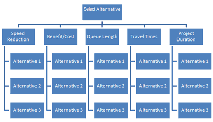
There are a variety of different weighting/scoring methods that can be applied in a work zone MOTAA process. Most take a common structure such as that depicted in Figure 18. Where the approaches tend to differ is in the establishment of criteria weights and how those weights are used to choose a recommended alternative. Some of the most common approaches in these weighting/scoring techniques are based in Multi-Criteria Decision-Making Models (MCDM). Using mathematical methodologies that assign weight to criteria, MCDM models enable analysts to evaluate and compare the utility or relevancy of criteria or factors to a problem. There are a variety of MCDM models that can be applied for work zone MOTAA. The more common MCDM models used for various decision-making applications include weighted sum model, weighted product model, analytical hierarchy process, ELECTRE, and TOPSIS. For the purpose of this guide, two MCDM models will be discussed in further detail. The two models are the weighted sum model or simple additive weighting and analytical hierarchy process (AHP). The weighted sum is typically deemed the simplest of the MCDM models and AHP is one of the most commonly used MCDM models for decision-making.
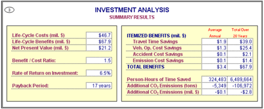
Additional weighting or scoring techniques that can be applied for evaluating alternatives include Kepner-Tregoe Method and Benefit/Cost Analysis. Kepner-Tregoe Decision Methodology can be used for gathering, prioritizing and evaluating information. It also incorporates ranking and scoring within its decision-making framework. Benefit/cost analysis is an economic decision-making approach that weighs and values an alternative’s expected benefits and costs. A benefit/cost analysis can generate Benefit/Cost ratios (B/C ratios) that can be used to compare and choose amongst alternatives.
Figure 18. Weighting/Scoring Technique Framework
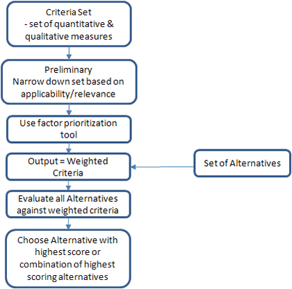
Table 56 summarizes the various features and capabilities of the different weighting and scoring techniques. More details on each tool can be found in the subsections that follow.
Table 56. Evaluation Tools and Methods for Comparing Alternatives
| Methods/Considerations |
Project Complexity Suited For |
Analysis Complexity |
Level of Data Needs |
Development Time |
Analysis Time |
Number of Criteria Elements |
| Traditional |
Low-Medium |
Low |
Medium |
Low |
Low |
Low |
| Simple Additive Weighting (SAW) |
Low-Medium |
Low |
Medium |
Low |
Medium |
Medium |
| Analytical Hierarchy Process |
Medium-High |
High |
Medium |
Medium |
High |
High |
| Kepner Tregoe Method |
Medium-High |
High |
High |
High |
High |
High |
| Benefit/Cost |
Medium-High |
Medium |
High |
High |
Medium |
High |
MCDM Models – Weighted Sum Method or Simple Additive Weighting (SAW)
The weighted sum method is commonly deemed as the more simple of the MCDM models. The weighted sum states that if there are m alternatives and n criteria, an alternative’s score is determined using the following equation:

Where:
Si = The SAW score of the alternative;
aij= The ith alternative’s score for the jth criterion; and
wj= The weight of the jth criterion.
In this method, the decision-maker must accomplish two tasks prior to applying SAW. The first is to determine the criteria weights and the other is to develop a way to obtain each alternative’s relevancy scores. Once these two tasks have been completed, the decision-maker can apply the SAW equation to each alternative to calculate their weighted scores. The alternative that scores the highest is typically recommended.
Example Application of SAW
To evaluate and choose amongst a set of work zone alternatives using the SAW method, the decision-maker can take the following steps:
- Step 1 – The evaluator or analyst decides to use the weighted criteria using the ranking method (see Section 5.2).
- Step 2 – The analyst assembles a panel of decision-makers that will score the alternatives based on how well they meet the criteria elements. The evaluator asks them to score the alternatives (e.g., such as the scale shown in Table 57).
- Step 3 – The analyst averages the scores for each alternative by criterion. The SAW equation is applied to determine the final weighted score for each alternative. The final scores are shown in Table 58. In this example, Alternative 2 scores the highest and is recommended.
Table 57. Example Score for Alternatives
| Scale for Scores |
| Most Effective |
30 |
| Mediocre |
20 |
| Not Effective |
10 |
Table 58. SAW Example
| Alternative |
Criteria and Weights |
Speed Reduction Potentials
0.27 |
Capital and O&M Costs
0.33 |
Queue Length
0.20 |
Travel Times
0.13 |
Project Duration
0.07 |
Score |
| 1 |
25 |
20 |
15 |
30 |
15 |
21.30 |
| 2 |
10 |
30 |
20 |
30 |
30 |
22.60 |
| 3 |
30 |
10 |
30 |
10 |
10 |
19.40 |
Table 59. Pros and Cons of SAW
| Pros |
Cons |
- Simple analysis.
- Applicable to various problems.
- Does not have to be too resource intensive. It does not require additional tools or software, or personnel with technical backgrounds.
|
- Requires polling a group of people for their opinion on ranking or score, which could be time-consuming.
- Assigning of rankings/scores are subjective and are not necessarily required to be justifiable based on field data, market research, expert panels, recorded observations, etc.
|
MCDM Models – Analytical Hierarchy Process (AHP)
The Analytical Hierarchy Process (AHP) is an MCDM decision-making approach that utilizes a multiple choice criterion that is structured in a hierarchical format. It involves assessing the relative importance of the criteria (assigning criteria weights), comparing alternatives for each criterion, and determining an overall score or ranking for the alternatives.
Example Application
This example demonstrates how an AHP can be used to evaluate and choose amongst work zone alternatives. The following outlines the preliminary steps in beginning an AHP analysis:
- Step 1 – Determine the objective of the analysis: In this case, it is “To choose the preferred alternative amongst three potential choices.”
- Step 2 – Define the criteria: Speed Reduction Potentials, Capital and O&M Costs, Queue Length, Travel Times, and Project Duration.
- Step 3 – Determine a set of alternatives. For this example, the alternatives will be labeled as: Alternatives 1, 2, and 3.
- Step 4 – Arrange the information in a hierarchical format (e.g., Figure 19).
- Step 5 – Use pairwise comparisons to determine the criteria weights. Similar to the Paired Comparison Analysis, the pairwise comparison in the AHP measures the importance of one criterion relative to another. An example is shown in Table 60.
Figure 19. AHP Hierarchical Tree Example

Table 60. Pairwise Comparison Matrix
 |
Speed Reduction Potentials |
Capital and O&M Costs |
Queue Length |
Travel Times |
Project Duration |
| Speed Reduction Potentials |
1/1 |
4/5 |
4/3 |
4/2 |
4/1 |
| Capital and O&M Costs |
5/4 |
1/1 |
5/3 |
5/2 |
5/1 |
| Queue Length |
3/4 |
3/5 |
1/1 |
3/2 |
3/1 |
| Travel Times |
2/4 |
2/5 |
2/3 |
1/1 |
2/1 |
| Project Duration |
1/4 |
1/5 |
1/3 |
1/2 |
1/1 |
- Step 6 – Turn the pairwise comparison matrix into a prioritization matrix using eigenvector. In order to do this, the matrix shown in Table 60 must be converted into its decimal values, as shown in
Table 61. Pairwise Matrix in Decimal Form
 |
Speed Reduction Potentials |
Capital and O&M Costs |
Queue Length |
Travel Times |
Project Duration |
| Speed Reduction Potentials |
1.00 |
0.80 |
1.33 |
2.00 |
4.00 |
| Capital and O&M Costs |
1.25 |
1.00 |
1.67 |
2.50 |
5.00 |
| Queue Length |
0.75 |
0.60 |
1.00 |
1.50 |
3.00 |
| Travel Times |
0.50 |
0.40 |
0.67 |
1.00 |
2.00 |
| Project Duration |
0.25 |
0.20 |
0.33 |
0.50 |
1.00 |
- Step 7 – Square and normalize the matrix. The matrix in Table 61 is squared to generate the new matrix shown in Table 62. The row sum and row total (sum of the row sum) are calculated. The values are normalized by dividing the row sum by the row total. The final column in Table 62 represents the eigenvector.
- Step 8 – Iteratively square the matrix. The matrix from Table 62 (columns Speed Reduction through Project Duration) is squared once more and a new set of eigenvectors is generated. The analyst is recommended to go through multiple iterations of this process until the eigenvector solution does not change from the previous iteration.
Table 62. Generating the Eigenvector
 |
Speed Reduction Potentials |
Capital and O&M Costs |
Queue Length |
Travel Times |
Project Duration |
Total |
Normalize
(Row Sum/Row Total) = EIGENVECTOR |
| Speed Reduction Potentials |
1.00 |
0.64 |
1.78 |
4.00 |
16.00 |
23.42 |
0.2909 |
| Capital and O&M Costs |
1.56 |
1.00 |
2.78 |
6.25 |
25.00 |
36.59 |
0.4545 |
| Queue Length |
0.56 |
0.36 |
1.00 |
2.25 |
9.00 |
13.17 |
0.1636 |
| Travel Times |
0.25 |
0.16 |
0.44 |
1.00 |
4.00 |
5.85 |
0.0727 |
| Project Duration |
0.06 |
0.04 |
0.11 |
0.25 |
1.00 |
1.46 |
0.0182 |
| Total |
80.50 |
1.00 |
- Step 9 – Check for matrix stability. After several iterations, the eigenvectors stabilize to the values listed in Table 63. These values represent the criteria weights.
Table 63. Criteria Rankings/Weights
 |
Ranking |
| Speed Reduction Potentials |
0.2907 |
| Capital and O&M Costs |
0.4543 |
| Queue Length |
0.1634 |
| Travel Times |
0.0725 |
| Project Duration |
0.0180 |
- Step 10 – Generate the pairwise comparisons. This pairwise comparison for the alternatives is used to determine the preference of each alternative over the other relative to the criterion. Table 64 shows the pairwise comparisons for the alternative for criterion, Speed Reduction Potentials.
Table 64. Pairwise Comparison of Alternatives
| Alternative |
Speed Reduction Potential |
| Alternative 1 |
Alternative 2 |
Alternative 3 |
| 1 |
1.00 |
2.00 |
3.00 |
| 2 |
0.50 |
1.00 |
2.00 |
| 3 |
0.33 |
0.50 |
1.00 |
- Step 11 – Compute the eigenvector of each alternative for each criterion and select the preferred alternative. As shown in Table 65, to generate the final score of each alternative, the alternative rankings are multiplied by the criteria weights. In this example, Alternative 2 scores the highest and is chosen.
Table 65. AHP Final Score and Recommendation
| Alternative |
Speed Reduction Potentials
0.2907 |
Capital and O&M Costs
0.4543 |
Queue Length
0.1634 |
Travel Times
0.0725 |
Project Duration
0.0180 |
Final Score
(Criteria Ranking Alternative Ranking) |
| 1 |
0.3846 |
0.3333 |
0.2308 |
0.4286 |
0.2727 |
0.3370 |
| 2 |
0.1538 |
0.5000 |
0.3077 |
0.4286 |
0.5455 |
0.3631 |
| 3 |
0.4615 |
0.1667 |
0.4615 |
0.1429 |
0.1818 |
0.2990 |
Table 66. Pros and Cons of AHP
| Pros |
Cons |
- Applicable to various problems.
- Does not have to be too resource intensive. It does not require additional tools or software, or personnel with technical backgrounds.
- Checks the consistency of evaluation measures and alternatives in an effort to reduce bias.
|
- Requires polling a group of people for their opinion on ranking or score, which could be time-consuming.
- Determining the eigenvectors, if done manually, could be time-consuming as well.
- Different hierarchical structures could lead to different results.
- Pairwise comparison – limited comparability.
- Rank reversal – depending on how the question is framed may get different results.
|
Kepner-Tregoe (KT) Method
The Kepner-Tregoe decision-making methodology can be used for prioritizing and evaluating alternatives. The method features a step-by-step approach that can aid a decision-maker to choose amongst alternatives by evaluating each of their impacts, risks, and opportunities. It typically involves the following steps:
- Preparing the Decision Statement – This establishes the objectives, the desired result, and the action required.
- Defining the Objectives – At this step, the objectives are classified according to their relative importance as “musts” and “wants.” Certain objectives will be considered mandatory and will, therefore, be considered as “musts.” Those that are desirable will fit into the “wants” category.
- Ranking the Objectives and Assigning Relative Weights – At this step, “wants” objectives are ranked on a 1 through 10 scale, where rank 10 is considered most important and 1 is least important.
- Listing Alternatives – At this stage, a list of potential alternatives are brought into the analysis.
- Evaluating the Alternatives – The alternatives are evaluated based on the “must” and “wants” objectives. The first step in evaluating the alternatives is to eliminate those that do not fit the “must” or mandatory objectives. The remaining alternatives are then scored by how they meet the “wants” objectives. The alternatives are rated against each “wants” objective on a scale of 1 through 10, where 10 means the alternative best satisfies the “want.” The final score for each alternative will be a weighted value calculated by multiplying the “want” objective’s weight times the alternative’s satisfaction score.
- Choosing the Top Alternatives – After Step 5 has been exercised for all of the alternatives, the top two or three may be considered for the next stage where the alternatives are rated against potential future adverse effects.
- Evaluating the Alternatives against Potential Negative Effects – In this step, a set of potential consequences will be generated. The impact of each consequence will then be determined by evaluating the probability of it occurring and the severity of the impact should this event occur. The probability and impact scores are again determined on a 1 through 10 scale, where 10 is highest probability of occurrence or most serious degree of impact.
- Choosing the Preferred Alternative – The preferred alternative will be the one that satisfies the “must” objectives, scores the highest on the “wants” objectives analysis, and provides best potential to minimize the adverse impacts.
Example Application
The following example is derived from the Work Zone Road User Costs – Concepts and Applications. (Work Zone Road User Costs – Concepts and Applications. Federal Highway Administration, U.S. Department of Transportation, FHWA-HOP-12-005, December 2011.)
Step 1 – Prepare Decision Statement
The KT decision analysis process begins with a precise statement of what needs to be done (i.e., the purpose or the intended result) and how it will be done (i.e., actions required). This statement provides the focus for all other steps that follow and sets the limits on the range of alternatives that would considered in the decision analysis. This statement must be defined consistent with the work zone-related agency policies and project-specific needs.
The decision statement for a hypothetical project “Pavement Reconstruction of U.S. 00” is presented as follows:
Example 1
U.S. 00 serves as a major arterial road connecting the regional industrial hub with the twin metros. The pavement has reached its useful life and needs major reconstruction. The route carries significant amounts of commuter and truck traffic. The alternative routes for the detour have limited lane capacity and can accommodate only a portion of the work zone traffic volume.
Decision Statement
The purpose of the decision analysis is to identify the most appropriate strategy for maintaining traffic on U.S. 00 during the reconstruction of the pavement segments between Mileposts 100 and 105.
Step 2 – Define Objectives
The objectives are the decision criteria that describe the required and desired attributes of the resulting choice, and the explicit limits imposed on the decision process. The objectives include:
- MUSTS – These are the mandatory attributes required for an alternative to be considered in the decision process. These attributes are considered mandatory to guarantee a successful decision. Any alternative that cannot comply with a MUST objective is eliminated for further consideration, while those that comply with all the MUST objectives qualify as feasible alternatives. The MUST objectives should be measurable and provide an absolute GO/NO GO judgment.
- WANTS – These are the desired attributes based on which preferred alternative is selected from the pool of feasible alternatives (i.e., alternatives that fulfill all the MUST objectives). A mandatory or high-priority objective can be considered as a WANT objective, if that objective is not measurable or a relative assessment is preferred over an absolute GO/NO GO judgment. A MUST objective also can be considered as a WANT objective by rephrasing the objective statement for relative assessment of feasible alternatives.
In other words, the MUSTs decide who gets to play, but the WANTS decide who wins.
A list of MUST objectives for the “Pavement Reconstruction of U.S. 00” example is presented as follows:
- Maintain a minimum of one lane each direction for work zone traffic during weekday peak hours
Go/No Go
- No lane closure between 7:00 a.m. through 10:00 a.m.and 4:00 p.m. through 8:00 p.m. during weekdays
Go/No Go
- Queue length not more than 0.75 miles for more than one hour
Go/No Go
- Delay time not more than 30 minutes
Go/No Go
- Alternative detour route exceeds capacity?
Go/No Go
A list of WANT objectives for the example is presented as follows:
- Minimize daily road user costs ($)
- Minimize number of days for project completion
- Minimize traffic control and construction engineering costs ($)
- Minimize length of detour (miles)
- Minimize queue length (lane-miles)
- Minimize average delay time per vehicle (minutes)
- Minimize percent motorist traveling at a speed 15 mph less than the posted limit
- Minimize average time to clear a noninjury incidence (minutes)
- Maintain emergency services (adjectival ratings – poor, average, good)
- Reduce environmental impacts (adjectival ratings – low, moderate, severe)
Selection of Objectives
One of the commonly cited concerns with a decision analysis is the interdependency among objectives. It is a phenomenon where two or more objectives are highly correlated. The presence of interdependence among objectives in a decision analysis can produce erroneous or misleading outcomes. Interdependence leads to double counting and tends to weigh heavily toward the interdependent factors, while diminishing the significance of other factors in the analysis. Therefore, it is imperative that a decision analyst screen for interdependency among the objectives and validate them.
For example, consider the list of WANT objectives presented above. The factor “daily road user costs” is highly correlated with the following factors: length of detour, maximum queue length, average delay time, average time to clear noninjury incidence, and percent traveling at a speed 15 mph less than the posted speed limit. These factors all contribute to the computation of the daily road user cost value. Similarly, the factors “the number of days for project completion” and “traffic control and construction engineering costs” also are highly correlated.
One common technique used by practitioners in screening the interdependency among objectives is sensitivity analysis. A sensitivity analysis can be conducted formally or informally to evaluate the effects of varying one objective (numerical or adjectival) on other objectives and final outcomes. The results of the sensitivity analysis will help to identify correlations among analysis factors. Both the degree of correlation and the logical dependency between the factors should be taken into account while identifying the dependent pairs. The purpose here is to avoid double counting rather than eliminating all correlated factors.
Consider the dependency between two pairs: 1) average delay time versus daily road user cost; and 2) average delay time versus average time to clear a noninjury incidence. In the former case, considering both the factors in the analysis will lead to double counting as the factor “daily road user cost” is a monetized aggregation of various impacts, including the factor “average delay time.” Any change in the average delay time will result in a proportional change in the daily road user cost. In such cases, it is suggested to eliminate the factor “average delay time” or break the factor “daily road user cost” into individual components.
In the latter case, the factor “the change in average time to clear a noninjury incidence” also causes a proportional change in the average delay time and, hence, is highly correlated. However, considering the probability of a noninjury incidence and the importance of clearing the incident, the analyst may prefer to list both factors to emphasize the effectiveness on traffic incident management in MOT alternative selection and to distinguish it from other traffic delay control strategies. Therefore, it is imperative to use engineering judgment and experience in selecting the objectives so that the intended purpose of the analysis and the complexity of the problem are not diluted.
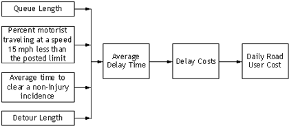
Interdependency can be countered effectively by defining the objectives in near similar hierarchical order. The problem of interdependency may occur if one objective is defined at the aggregate/generic level while another is defined at the component/specific level. For example, in the list of WANT objectives presented above, the interdependency between the factor “daily road user cost” and other factors is a result of mixing up the factors from different hierarchical order, as illustrated in Figure 20. This figure presents the relationship between “daily road user costs” and only those delay-related WANT objectives listed in the example. The factors listed on the left (queue length, average time to clear a noninjury incidence, etc.) contribute in determining the average delay time which, is used in the daily road user cost computation.
Figure 20. Illustration of Relationships among Factors

A modified list of WANT objectives for the example is presented as follows:
- Minimize delay costs
- Minimize vehicle operating costs
- Minimize number of days for project completion
- Minimize traffic control and associated construction costs (e.g., shoulder widening, temp bridges), etc.
- Minimize average time to clear a noninjury incidence (minutes)
- Maintain emergency services (adjectival ratings – poor, average, good)
- Reduce environmental impacts (adjectival ratings – low, moderate, severe)
Step 3 – Weighting the Objectives
All MUST objectives are assigned with GO and NO GO options. Each WANT objective is weighted on a scale of 1 to 10 based on their relative importance in the decision process, with the weight of 1 indicating “least preferable” and 10 indicating “most preferable.” The weights assigned to the WANT objectives should reflect the agency’s work zone policies and project-specific needs.
The following issues should be evaluated while assigning the weights:
- Too many high weights may indicate either unrealistic expectations or a faulty perception of which objectives can guarantee success;
- Too many low weights suggest the possible inclusion of unimportant details in the analysis; and
- Biased objectives may produce an ineffective analysis.
The following illustrates the assigning of weights to each of the WANT objectives considered in the “Pavement Reconstruction of U.S. 00” example:
Step 3 – Weighting the Objectives
| No. |
WANT Objective |
Assigned Weight |
| 1 |
Delay costs |
10 |
| 2 |
Vehicle operating costs |
8 |
| 3 |
Number of days for project completion |
10 |
| 4 |
Traffic control and associated construction costs ($) |
8 |
| 5 |
Average time to clear a noninjury incidence (minutes) |
4 |
| 6 |
Maintenance of emergency services (adjectival ratings – poor, average, good) |
6 |
| 7 |
Environmental impacts (adjectival ratings – low, moderate, severe) |
3 |
(Source: Federal Highway Administration, 2011.)
Step 4 – Identify Candidate Alternatives
Identify all potential alternatives, whether immediately feasible or not, to be evaluated and measured as MUST and WANT objectives. Use the alternatives identified in Step 4 as candidate alternatives for decision analysis.
The candidate alternatives for the “Pavement Reconstruction of U.S. 00” example are listed as follows:
Daytime partial lane closure – closed between 7:00 a.m. to 5:00 p.m.
Nighttime partial lane closure – closed between 8:00 p.m. to 6:00 a.m.
Nighttime partial lane closure – closed between 9:00 p.m. to 7:00 a.m.
Nighttime full lane closure – closed between 9:00 p.m. to 6:00 a.m.
Truck traffic diverted through alternative detour routes during peak hours.
Step 5 – Summarize the Findings of Work Zone Impact Assessment
A detailed work zone impact assessment for each candidate alternative should be done to evaluate both MUST and WANT objectives for quantitative and qualitative results. Use the findings of the preliminary and detailed impact assessments for evaluation. The assessment findings should be summarized for each alternative against the objectives.
The following summarizes the impact assessment findings of all alternatives against the MUST objectives considered in the “Pavement Reconstruction of U.S. 00” example:
Step 5 – Summarize the Findings of Work Zone Impact Assessment
| MUST Objective |
Alternative Evaluation |
| A |
B |
C |
D |
E |
| Maintain a minimum of one lane each direction for work zone traffic during weekday peak hours |
Yes |
Yes |
Yes |
Yes |
Yes |
| No lane closure between 7:00 a.m. through 10:00 a.m. and 4:00 p.m. through 8:00 p.m. during weekdays |
No |
Yes |
Yes |
Yes |
Yes |
| Maximum queue length (miles) |
1.6 |
0.0 |
0.0 |
0.5
(Calculated for the selected detour route) |
0.5b
(Weighted average for both mainline and detour routes) |
| Average delay time per vehicle (minutes) |
19.0 |
6.0 |
3.0 |
10.0
(Calculated for the selected detour route) |
20.0
(Weighted average for both mainline and detour routes) |
| Alternative detour route exceeds capacity? |
No |
No |
No |
No |
Yes |
(Source: Federal Highway Administration, 2011.)
The following summarizes the impact assessment findings of all alternatives against the WANT objectives considered in the “Pavement Reconstruction of U.S. 00” example:
Step 5 – Summarize the Findings of Work Zone Impact Assessment
| WANT Objective |
Alternative Evaluation |
| A |
B |
C |
D |
E |
| 1. Delay costs |
$5,300 |
$3,125 |
$2,800 |
$4,700 |
$6,800 |
| 2. Vehicle operating costs |
$1,484 |
$656 |
$728 |
$1,175 |
$1,836 |
| 3. Number of days for project completion |
150 |
84 |
84 |
60 |
90 |
| 4. Traffic control & associated construction costs ($) |
$55,000 |
$94,000 |
$75,000 |
$109,000 |
$85,000 |
| 5. Average time to clear a non-injury incidence (minutes) |
20 |
25 |
25 |
15 |
10 |
| 6. Maintenance of emergency services (adjectival ratings – poor, average, good) |
Moderate |
Moderate |
Moderate |
Good |
Good |
| 7. Environmental impacts (adjectival ratings – low, moderate, severe) |
Moderate |
Severe |
Severe |
Low |
Low |
(Source: Federal Highway Administration, 2011.)
Step 6 – Evaluation of Alternatives against MUST Objectives
Evaluate all available alternatives against each of the MUST objectives identified in the earlier step. Any alternative is eliminated from further consideration if it fails to satisfy one or more of the MUST objectives; only those satisfying all the MUST objectives are considered as feasible alternatives.
The results obtained from the evaluation of alternatives against MUST objectives are presented as follows:
Step 6 – Evaluation of Alternatives against MUST Objectives
| MUST Objective |
Alternatives |
| A |
B |
C |
D |
E |
| Maintain a minimum of one lane each direction for work zone traffic during weekday peak hours |
Go |
Go |
Go |
Go |
Go |
| No lane closure between 7:00 a.m. through 10:00 a.m. and 4:00 p.m. through 8:00 p.m. during weekdays |
No Go |
Go |
Go |
Go |
Go |
| Queue length not more than 0.75 mile for more than one hour |
No Go |
Go |
Go |
Go |
Go |
| Delay time not more than 30 minutes |
Go |
Go |
Go |
Go |
Go |
| Alternative detour route exceeds capacity? |
Go |
Go |
Go |
Go |
No Go |
(Source: Federal Highway Administration, 2011.)
Outcome:
Alternatives A and E are eliminated.
Alternatives B, C, and D qualify as feasible alternatives.
Based on the evaluation results, Alternatives A and E are eliminated from further consideration as these alternatives did not satisfy all the required attributes. The remaining Alternatives B, C, and D are carried into the next step.
Step 7 – Evaluation of Alternatives against WANT Objectives
In this step, each alternative is assigned with a score of 1 to 10 against each WANT objective based on how well the alternative meets that objective. This step involves not only assessing each alternative individually against each WANT objective but also comparing the alternatives with each other against each WANT objective. The results obtained from the evaluation of alternatives against WANT objectives are presented as follows:
Step 8 – Weighting the Scores of Alternatives
The weighted score of each feasible alternative should be computed to determine the relative performance of the alternatives.
The weighted score is the score of an alternative multiplied by the weight of the WANT objective to which the score refers. For example, the weight of the objective “Length of detour” is 7 and the score of Alternative D against this objective is 2. Therefore, the weighted score of Alternative D on that objective is 14. For each alternative, all the weighted scores are added up to calculate the total weighted score for that alternative.
The total weighted score of an alternative indicates how well an alternative stacks up against each of the other alternatives for overall performance against WANT objectives. In other words, the total weighted scores function as a visible comparative performance of the alternatives.
For the “Pavement Reconstruction of U.S. 00” example, the individual and the total weighted scores of each feasible alternative are presented as follows:
(Source: Federal Highway Administration, 2011.)
In this example, Alternative D is considered as the tentative choice.
Step 9 – Evaluation of Adverse Consequences (Optional)
After the completion of the alternative evaluation using MUST and WANT objectives, the feasible alternatives can be further evaluated against potential risks. The objective of this step is to understand the consequences of selecting an alternative.
This step is deemed optional as the potential risks are expected to be identified in the work zone impact assessment and incorporated into the decision analysis as a MUST or WANT objective.
This step is particularly recommended when the total weighted scores of all the alternatives are closer. In the “Pavement Reconstruction of U.S. 00” example, the total weighted scores of alternatives B, C, and D are 373, 367, and 426, respectively. Since these scores are close, a risk assessment may be warranted to ensure that the best decision is being made. Suppose, if the total weighted scores of these alternatives were 100, 110 and 633, respectively, alternative D stands out among the feasible ones by an order of magnitude and, therefore, a risk assessment is not required.
The risk assessment begins with the tentative choice (i.e., the alternative with the highest total weighted score). For this alternative, the probability of an adverse consequence and the severity of the impact (i.e., performance of an alternative under that event) is assessed and rated on a High-Medium-Low scale or a scale of 10 (high probable/very severe) to 1 (unlikely/not severe). This step is repeated for each potential adverse consequence to produce the “adverse consequence totals.” The risk assessment is then repeated for other feasible alternatives.
For the “Pavement Reconstruction of U.S. 00” example, three potential risks were considered:
- Event of flooding;
- High severity crashes (involving multiple crashes and longer incidence time); and
- Event of an emergency evacuation due to a natural catastrophe.
The likelihood of these events occurring and the performance of an alternative under these situations were rated as probability and severity ratings, respectively. The weighted score for each risk factor is calculated to produce the total adverse consequence score of an alternative. The example is presented as follows:
Step 10 – Selection of the Preferred MOT Strategy
For each alternative, the net score is calculated by subtracting the total adverse consequence score from the total weighted score. The alternative with the highest net score is selected as the preferred MOT strategy.
In the “Pavement Reconstruction of U.S. 00” example, Alternative D (i.e., Nighttime full lane closure between 9:00 p.m. and 6:00 a.m.) is selected as the preferred MOT strategy.
Step 10 – Selection of the Preferred MOT Strategy
| Alternative |
Description |
Total Weighted Score |
Total Adverse Consequence Score |
Total Score |
Rank |
| A |
Daytime partial lane closure – closed between 7:00 a.m. to 5:00 p.m. |
Eliminated |
– |
– |
– |
| B |
Nighttime partial lane closure – closed between 8:00 p.m. to 6:00 a.m. |
373 |
-42 |
331 |
2 |
| C |
Nighttime partial lane closure – closed between 9:00 p.m. to 7:00 a.m. |
367 |
-42 |
325 |
3 |
| D |
Nighttime full lane closure – closed between 9:00 p.m. to 6:00 a.m. |
426 |
-59 |
367 |
1 |
| E |
Truck traffic diverted through alternative detour routes during peak hours. |
Eliminated |
– |
– |
– |
(Source: Federal Highway Administration, 2011.)
Table 67. Pros and Cons of Kepner-Tregoe Method
| Pros |
Cons |
- Applicable to various problems.
- Does not have to be too resource intensive. It does not require additional tools or software, or personnel with technical backgrounds.
- Accounts for some risk analysis.
|
- Requires polling a group of people for their opinion on ranking or score, which could be time-consuming.
- Still has some bias since individual or group must decide on the relevancy, probability, and severity scores.
|
Benefit/Cost Analysis
A benefit/cost analysis (BCA), though primarily based on financial information, can be used to compare and choose among alternatives. An agency can choose from various readily available tools or customize their own. There are a variety of tools created for transportation-related projects, including the FHWA’s HERS-ST, California DOT’s (Caltrans) Cal-B/C, and Texas Transportation Institute’s MicroBENCOST. Different B/C tools may be best fit for certain projects. The FHWA currently is working on developing a Benefit/Cost desk reference tool which will have a feature that will match the appropriate B/C tool to an agency’s project type and needs.
The B/C method typically includes the following steps:
- Step 1 – Identify and select the data for use in the BCA;
- Step 2 – Determine the benefits elements;
- Step 3 – Determine the cost elements; and
- Step 4 – Compare the sum of the costs with the sum of the benefits and determine a benefit/cost ratio.
For a work zone MOTAA analysis, there are several factors that can influence the benefit/cost analysis. Benefit elements that can be used in evaluating and comparing alternatives could include monetary value of travel time savings, road user cost reductions, emissions reductions, and other cost savings. Cost elements could include capital, operations and maintenance, and other costs and fees associated with the project. For more details on the specific work zone-related considerations that should be incorporated in a work zone MOTAA-specific BCA, please refer to Chapter 6 of this document. For additional information on how to calculate specific work zone-related costs, please refer to Work Zone Road User Costs – Concepts and Applications. (Work Zone Road User Costs – Concepts and Applications. Federal Highway Administration, U.S. Department of Transportation, FHWA-HOP-12-005, December 2011.)
Example Application
- Step 1 – The first step in a benefit/cost analysis for a work zone project would be to determine relevant project information that would serve as input data for the BCA. Such input data could include:
- Project Characteristics – Length of construction period, project type, and length of peak period affected;
- Design and Traffic Information – Work zone strategy (i.e., lane closure, corridor reconstruction, etc.), average daily traffic, speeds, and vehicle make-up of traffic; and
- Safety and Accident Statistics – Fatal and injury accident rates.
- Step 2 – The benefits for the project alternative are calculated using the selected analysis tool. The performance measures are monetized based on the value of each performance measure. These benefits are typically calculated over the lifetime of the project and are brought to a Net Present Value (NPV).
- Step 3 –The project costs information are determined by looking at all direct costs associated with construction, operations and maintenance of the project alternative, as well as additional costs associated with any mitigation measures needed. The costs are typically calculated over the lifetime of the project and are discounted to a NPV.
- Step 4 – The results of the analysis will produce the total NPV of the benefits and costs of the project. Typically a Benefit/Cost ratio is determined as a common measure to compare different project alternatives. The B/C ratio is determined by dividing the total benefits by the total costs of the alternative. This process is conducted for all alternatives. The alternative with the best B/C ratio should be chosen as the preferred alternative. For reference, a summary results sheet from one BCA tool, Cal-B/C, is shown in Figure 21. (System Metrics Group, Inc., and Cambridge Systematics, Inc. California Life-Cycle Benefit/Cost Analysis Model (Cal-B/C) User’s Guide (Version 4.0). California Department of Transportation, February 2009.)
Figure 21. Benefit/Cost Analysis Summary Results Example

Table 68. Pros and Cons of Benefit/Cost Analysis
| Pros |
Cons |
- Applicable to various problems
- Accounts for costs, risks, and performance – all critical to determining the feasibility of the alternative
- Based on data that is verifiable through field data, case studies, etc.
|
- May be data intensive
- Could provide erroneous results if calculations, forecasts, and estimates are unrealistic
- Benefits and cost elements included in the analysis are subject to the analyst or decision-maker(s)
- Some benefits or costs may not be easily quantifiable
|
5.4 Decision-Making Tools for Work Zone Alternatives Analysis
The previous sections described how to prioritize and establish criteria weights and then use those weighted criteria in a decision-making evaluation framework to evaluate and choose among potential alternatives. This section will provide information on various tools that automate or package decision-making analysis methods into a readily available tool or software. The section is structured as follows:
- Overview of the methodology/tool, including application steps;
- Additional considerations, including pros and cons; and
- Case study of tool application for work zones.
Knowledge-Based Systems (Case-Based Reasoning)
Overview of Methodology/Tool
Case-based reasoning (CBR) is a methodology for storing and retrieving previous cases and adapting them to a new solution. A case-based reasoning system is one methodology for solving problems that uses prior knowledge to adapt new solutions. The CBR framework featured in this section is based upon the CBR model developed by Karim and Adeli (2003) for work zone traffic management. (Karim, A., and H. Adeli. CBR Model for Freeway Work Zone Traffic Management. Journal of Transportation Engineering, Volume 129, No. 2, March/April 2003, pages 134-145.)
Typical components of a CBR are illustrated in Figure 22. (Karim, A., and H. Adeli. CBR Model for Freeway Work Zone Traffic Management. Journal of Transportation Engineering, Volume 129, No. 2, March/April 2003, pages 134-145.) The following sections provide further explanation on how each of these elements can be applied to a work zone traffic management example. The use of CBR for work zone MOTAA analysis differs from the other decision methods because unlike the other frameworks, the agency does not have to create a preliminary list of potential alternatives. If there is a sufficient database that supports the CBR tool, the outputs of the analysis should present the optimal alternative(s) based on the project characteristics inputs and the weights set by the agency analyst.
Case Models for the Work Zone Traffic Management – Domain Information
The domain information serves at the base of CBR, providing a structure for the problem identification and formulation and also the collection of experiences that will serve as references for the solution and calculation of impacts. Karim and Adeli’s research sets to explain the use of the CBR system for work zone traffic management through a four-set case model that consists of the following:
- General – The general set contains information that provides historical information and previous experiences for future reference.
- Problem – The problem set includes information that defines the constants of the work zone traffic control problem. This set typically contains project characteristics.
- Solution – The solution set contains information regarding the work zone layout, strategies, and traffic mitigation measures.
- Effects – The effects set contains information about the traffic impacts for the work zone.
Figure 23 provides an example of the data components and work zone parameters considered within the four-set case model. (Karim, A., and H. Adeli. CBR Model for Freeway Work Zone Traffic Management. Journal of Transportation Engineering, Volume 129, No. 2, March/April 2003, pages 134-145.)
Figure 22. Elements of CBR

(Source: Karim and Adeli, 2003.)
Figure 23. Four Set Case Model – Work Zone Example

(Source: Karim and Adeli, 2003.)
Case Representation
The second element of CBR is representation, which defines a data structure for the collected experiences or cases stored as reference. The type of representation used in this CBR research is attribute-value. The attribute-value system consists of three elements: attribute field name, attribute type, and value.
Case Retrieval
Another element of CBR is retrieval, which is the retrieval of a potential solution and determining similarities between the problem and previous cases. In the CBR system, retrieval starts with the formulation of a query. Based on this query, the system retrieves cases that can serve as potential solutions to the problem. These cases are retrieved due to their match or degree of similarity to the query/problem.
Factor Prioritization and Criteria Weights
The use of criteria weights is explained in further detail in the example application section. Weights can be determined using the factor prioritization methods detailed in the previous section.
Evaluation of Criteria Scores and Recommending an Alternative
As previously mentioned, cases are retrieved from a series of queries. The cases retrieved are ranked based on a similarity score that denotes how similar the case is to the reference case. In the CBR system, the level of similarity or similarity score ranges from 0 to 1, where 0 indicates no similarity and 1 means full similarity. The cases retrieved are ranked and presented to the user. The case with the highest score serves as the potential solution. Additionally, the evaluator can modify this case to better fit the reference case or the project objective.
Table 69. Pros and Cons of the CBR Tool
| Pros |
Cons |
- Tool is simple and user-friendly
- Provides a database of and case studies of work zone strategies
|
- Can require a lot of data
- There may not be enough case data available
- Development of tool and database modules could become complex
|
Example Application
The procedure for the creation of work zone traffic control plans using the CBR system for work zone traffic management is shown in Figure 24. (Karim, A., and H. Adeli. CBR Model for Freeway Work Zone Traffic Management. Journal of Transportation Engineering, Volume 129, No. 2, March/April 2003, pages 134-145.) When a traffic analyst decides to create a traffic control plan for a given work zone scenario, the analyst begins with basic project information, such as number of lanes and flow rate. This background information is fed into the CBR system by responding to queries made by the system. The queries are done iteratively until the best fit case is found. The first query may start with basic information, such as number of lanes and the flow rate. To narrow down results further, additional queries can be made with other information about the work zone, such as phase duration or work zone intensity.
Figure 24. Work Zone Traffic Control CBR System

(Source: Karim and Adeli, 2003.)
The traffic analyst also can assign weights to certain attributes to further filter results based on priority or mandatory work zone characteristics. Finally, after the queries and weights have been applied, the analyst can compare the final results to each other based on their similarity scores. The higher the score indicates a closer match to the reference case and weights inputted by the user.
Additionally, the CBR system can evaluate the final list of cases retrieved and measure their impacts on motorists, the number and type of traffic control measures, and the maintenance of traffic cost. The best fit case or the case with the highest score can, therefore, provide insight regarding some potential work zone alternatives and mitigation strategies that could optimize the reference project’s operations and benefits. The CBR analysis will allow the analyst to modify their reference case/project with a desired solution or set of alternatives. The agency also can modify an existing case to obtain an improved solution or set of alternatives that will enable them to meet their particular goals, objectives, and/or criteria. Figures 25 to 25 provide snapshots of the CBR system used for work zone analysis following the four sets: General, Problem, Effects, and Solution. (Karim, A., and H. Adeli. CBR Model for Freeway Work Zone Traffic Management. Journal of Transportation Engineering, Volume 129, No. 2, March/April 2003, pages 134-145.)
Figure 25. CBR System General Set

(Source: Karim and Adeli, 2003.)
Figure 26. CBR System Problem Set

(Source: Karim and Adeli, 2003.)
Figure 27. CBR System Effects Object

(Source: Karim and Adeli, 2003.)
Figure 28. CBR System Solution Set

(Source: Karim and Adeli, 2003.)
Matrix-Based Decision Support Tool
Overview of Methodology/Tool
The Matrix-Based Decision Support Tool was created through a study funded by the FHWA and Texas Transportation Institute to determine the most effective strategies or combination of strategies to support construction, traffic management, and public information during work zone activities in high-traffic environments. (Carson, J.L., S.D. Anderson, and G.L. Ullman. Matrix-Based Decision Support Tools for Construction Activities on High-Volume Roads. In Transportation Research Record: Journal of the Transportation Research Board, No. 2081, Transportation Research Board of the National Academies, Washington, D.C., 2008, pages 9-28.) The research presents a series of decision-support matrices that include:
- Preliminary strategy selection matrix;
- More detailed matrices focused on construction, traffic management, and public information strategies; and
- An interdependency matrix that considers synergy among multiple strategies.
The use of these three matrices lends to a three-step process. To develop this process, the authors used information from literature reviews, case studies, and opinions of experts. Using the literature review and case studies, they developed the Preliminary Strategy Selection Matrix. This matrix maps the observed successful use of various construction, traffic management, and public information strategies. Using the literature review and case studies, they also gathered information regarding the benefits of each strategy. Using the benefits information, they developed the second matrix, the Secondary Strategy Selection Matrix. Separate matrices were developed for each of these three categories of strategies: construction, traffic management, and public information. Using the information sources, the researchers also observed that several of the strategies that were applied concurrently have synergic benefits. From the information regarding the different levels of synergy among strategies, the researchers created the third matrix, the Strategy Interdependency Matrix.
Preliminary Screening of Alternatives
Preliminary Strategy Selection Matrix
The Preliminary Strategy Selection Matrix presents various motivations or concerns related to construction, traffic management, and public information. It then identifies which strategies have been shown to mitigate or address such concerns using the three data sources previously mentioned. This matrix only identifies those strategies that positively address the associated motivations/concerns. Blank cells mean a negative or an unconfirmed positive relationship between the strategies and motivations/concerns.
Factor Prioritization and Criteria Weights
No factor prioritization methodology is necessary for this evaluation framework. However, the next strategy selection matrix aids the decision-maker to further reduce the set of strategies in consideration.
Secondary Strategy Selection Matrix: Construction
There are three Secondary Strategy Selection Matrices: 1) construction; 2) traffic management; and 3) public information. This secondary matrix provides additional information regarding the relative impacts and benefits of each strategy and rates them as either a high, medium, or low impact. The Secondary Matrix categorizes strategies into the following: contract administration, planning/scheduling, project management, constructability, and construction practices. It uses project examples from the case studies and identifies which strategies apply to which projects. It also identifies the anticipated benefits of each strategy as it relates to:
- Enhanced communications/coordination;
- Project speed and efficiency;
- Construction quality; and
- Work zone safety.
Evaluation of Criteria Scores and Recommending an Alternative
The three matrices work to decrease the initial set of strategies to those with a high level of relevance or significance to the project and the objectives. Additionally, the inclusion of the interdependency matrix also can provide insight into the optimal combination of strategies that could address the project objectives.
Strategy Interdependency Matrix
The third matrix, Strategy Interdependency Matrix, depicts the level of interdependencies between strategies. The interdependency levels are rated High, Medium, or Low. Similar to the Preliminary Strategy Selection Matrix, the Strategy Interdependency Matrix only identifies those combinations that have been shown to produce positive benefits. Therefore, blank cells reflect a disbenefit or an unconfirmed positive combination of strategies.
Table 70. Pros and Cons of the Matrix-Based Decision Support Tool
| Pros |
Cons |
- Simple and comprehensible for technical analysts, planners, and policy-makers
- Provides insight into optimal combination of strategies
- Database of benefits and case studies of work zone strategies
|
- Requires a lot of data
- Data for all strategies may not be available
- Narrows down strategies and denotes relevant strategies, but does not specifically recommend an alternative(s)
|
Example Application
Application of the matrices involves a three-step process that utilizes tables such as those shown in Figures 29 to 31. (Carson, J.L., S.D. Anderson, and G.L. Ullman. Matrix-Based Decision Support Tools for Construction Activities on High-Volume Roads. In Transportation Research Record: Journal of the Transportation Research Board, No. 2081, Transportation Research Board of the National Academies, Washington, D.C., 2008, pages 9-28.) The process is explained in further detail below.
- Step 1 – Preliminary Identification of Candidate Strategies – Use the Preliminary Strategy Selection Matrix to identify the appropriate strategies to address project considerations in the areas of construction, traffic management, and public information. The items included in the matrix’s top column labeled “Motivations/Concerns” can be used to guide project considerations.
- Step 2 – Further Investigation of Candidate Strategies – Use the Secondary Strategy Selection Matrix: Construction, Traffic Management, and Public Information Matrices to obtain more information about the candidate strategies generated from Step 1. This step provides further insights into the benefits and disbenefits of each strategy. Using the information from this matrix, the user can further narrow down their list of strategies to those that would provide benefits over a certain threshold or impact level.
- Step 3 – Identification of Synergistic Opportunities Among Candidate Strategies – After consolidating the initial list of strategies in Step 2, the third matrix, Strategy Interdependency Matrix, can be used to determine the optimal combination of strategies based on synergistic levels as a guide.
Figure 29. Preliminary Strategy Selection Matrix

Figure 30. Example Secondary Strategy Matrix: Construction

Fig 31. Level of Interdependence Matrix

PDF files can be viewed with the Acrobat® Reader®.

![]()
