3. Results and Findings
3.1 Crossing Characteristics
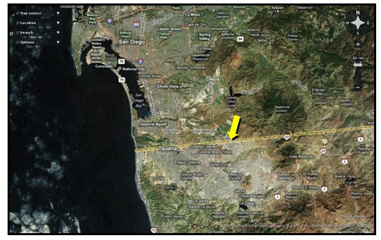
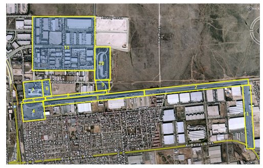
The Otay Mesa International Border Crossing is a truck-only crossing connecting the San Diego, California metro area with the city of Tijuana in the Baja California Peninsula. The Otay port of entry (POE), coupled with the adjacent San Ysidro crossing that serves automobile traffic, represents a key international trade transportation link. With more than 1.4 million truck crossings per year, the Otay Mesa Port of Entry is the largest commercial crossing in the California/Mexico border and handles the second highest volume of trucks and third dollar value of trade among all U.S./Mexico land border crossings.4 The satellite image in Figure 1 illustrates the location of the crossing.
Figure 1. Satellite Image of Otay Mesa Border Crossing Location
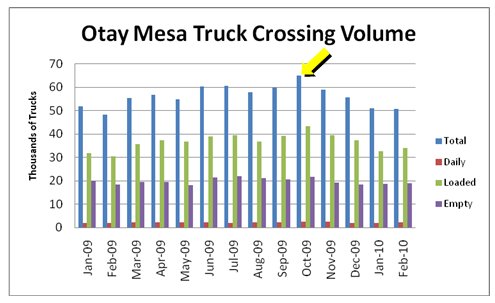
At the onset of the project, US Customs and Border Protection (CBP) staff at the Otay Mesa commercial crossing reported processing approximately 2,500 trucks per day during peak season, which runs from October through December. Figure 2 shows the actual volume of trucks that crossed through Otay Mesa into the US during the period between January 2009 and February 2010.5 As the figure indicates, the 2009 peak occurred in October, during which a total of nearly 65,000 trucks crossed from Mexico.
Figure 2. Otay Mesa Truck Crossings – January 2009 – February 2010
According to motor carriers, during the peak period each individual truck makes between 1.4 and 2 cross-border "turns" daily. The current layout of the Northbound crossing (from MX to the US) provides 1 FAST (Free and Secure Trade)6 lane, 2 laden lanes for general cargo, and 1 lane for empty trucks. This configuration starts at the "sorting gate" on the Mexican side of the crossing (see Figure 2), which is approximately 1.55 miles from the MX (Mexican) export facility and approximately 2 miles from the entry to the US Customs compound. FAST lanes process approximately 15 percent of total Northbound traffic (approximately 375 trucks per day during peak season). About one-third of Northbound movements are empty movements that cannot use FAST.
Otay Mesa is primarily a maquila crossing, where merchandise parts are shipped Southbound into the Tijuana area to be assembled and shipped Northbound into the US for delivery to distribution centers and retail stores. A substantial portion of peak season movements consist of electronics being shipped to the US for the Christmas holiday season. Motor carriers and US and MX customs staff note that traffic volume during this period is such that trucks crossing the international border often wait up to three hours. The second quarter (April to June) is the least busy from a truck volumes perspective, according to CBP staff, who indicate that wait times during this period are often 1 hour or less. Quarters 1 and 3 are moderately busy.
Border stakeholders report that Friday is the often busiest day at the crossing (more so during peak season), followed by Thursday, Monday/Tuesday, and Wed (in order of demand). Weekend hours and truck movements are more limited and represent some hazardous materials and Customs-Trade Partnership Against Terrorism (C-TPAT) movements only.
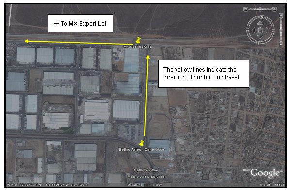
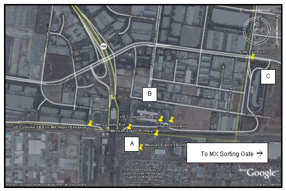
Motor carriers attending stakeholder sessions identified Northbound queues and respective border crossing travel times to characterize the Northbound movement. Figures 3 and 4 show the Northbound travel pattern. Figure 3 shows the approach from Mexico; Figure 4 includes customs facilities on both sides of the border as well as the California Highway Patrol (CHP) commercial vehicle safety inspection facility.
Figure 3. Google Earth Map of Northbound Access to Otay Crossing – MX
Mexican and US inspection facilities are shown in Figure 4 and are labeled as follows:
- A – Mexican Export Lot
- B – US Federal Inspection Facilities
- C – CHP: State Inspection Facility
The road connecting the MX sorting gate to MX customs serves is the location of the physical border.
Figure 4. Google Earth Map of Northbound Access to Otay Crossing (MX/US Customs Facilities and CHP Inspection Facility
During the stakeholder sessions, trucking company representatives and state and local government officials expressed interest in obtaining border travel time information across several distances:
- From the beginning of the queue at Calle Doce and Bellas Artes, through MX and US customs, to the exit of the CHP inspection facility. Motor carriers noted that this characterizes a complete cross-border trip. Additionally, from the intersection of Calle Doce and Bellas Artes, the travel time would likely extend beyond 3 hours.
- From the beginning of the queue to the MX sorting gate. In peak season, the cross-border queue often extends beyond Calle Doce and Bellas Artes. In off-peak, the MX sorting gate often marks the end of the queue.
- From the start of the queue to/through MX customs. A measure from the start of the queue to MX customs and then a measure of the time to traverse MX customs was of interest to both Aduana and US Customs and Border Protection (CBP) staff.
- At the exit of MX customs to/through US customs primary, allowing for a measure of wait times to enter customs as well as a measure of the time to traverse primary inspection. CBP officials noted that waits to traverse secondary inspection should not be included.
- From the exit of US customs primary to the exit of the CHP facility, with the CHP facility marking the end of the cross-border journey.
Table 1 summarizes the distances between these points of interest.
| Measurement Segment | Distance – Miles | |
|---|---|---|
| Image 1 | Bellas Artes at Calle Doce to MX Sorting Gate | 0.5 |
| Image 2 | MX Sorting Gate to MX Customs Primary | 1.55 |
| MX Customs Primary through MX Customs Exit | 0.2 | |
| MX Customs Exit to US Customs Primary | 0.3 | |
| US Customs Exit, through CHP inspection, to CHP Exit | 0.65 | |
| Total Distance (Estimated) Northbound | 3.2 |
Generally speaking, the roadway infrastructure between the Bellas Artes/Calle Doce intersection and the exit from the CHP safety facility has limited access, and at certain locations, has restrictive geometry. At the northern end of Calle Doce, the roadway turns 90 degrees to the left, and truck drivers are presented almost immediately with the sorting gate. Immediately downstream of the sorting gate the empty and FAST lanes are separated from the standard lanes by barriers. Trucks must then traverse the entire length of the roadway between the sorting gate and the MX export compound (a distance of approximately 1.55 miles) in this configuration.
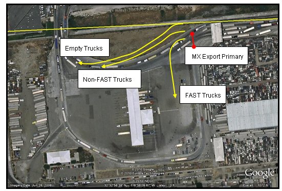
Upon arrival at and processing through the MX export facility, FAST trucks, which are in the leftmost lane, are routed south around the MX export secondary facility single-file, following a path just inside the perimeter of the compound. Empty trucks and non-FAST loaded trucks follow a route directly eastward to the exit at the northwest corner of the compound. The three truck types come together at this point, but remain in separate lanes-FAST trucks and bobtails (trucks without trailers) stay in a single lane to the left, loaded non-FAST trucks remain in the two middle lanes, and empty trucks stay in the lane to the right. An overhead view of the MX export compound is provided in Figure 5.
Figure 5. Satellite Image of Trucks Passing Through the Mexican Customs Export Compound
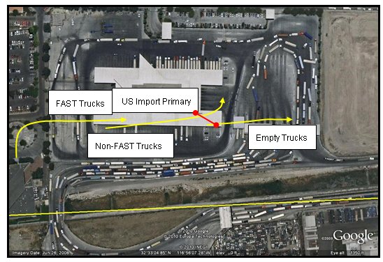
Once they pass across the border, trucks queue for entry processing into the US. Figure 6 contains an image of the US CBP entry processing facility. As the image shows, empty trucks follow a path parallel to the border from west to east, and do not enter the CBP compound. These vehicles are processed at a separate gate, at which CBP has an x-ray portal and a CBP officer stationed.
All other trucks must pass through the CBP primary screening facility and enter the US compound. FAST trucks are directed to the leftmost lanes. The two left lanes are dedicated to FAST traffic, and additional lanes can be used for FAST traffic as needed. Loaded trucks and bobtails must use one of the seven lanes to the right.
Figure 6. Satellite Image of Trucks Passing Through the US Customs Entry Compound
Once inside the US compound, trucks may be directed to do one of four different things:
- Proceed to the compound exit at the southeast corner of the compound by executing a u-turn near the northeast corner of the compound;
- Proceed to the secondary inspection facility at the center of the compound for further examination of cargo, paperwork, or driver credentials;
- Proceed in a loop around the secondary inspection facility to one of two x-ray screening portals on the west side of the compound; or
- Proceed straight ahead and form lines four abreast (called blocking) and await canine screening.
Which activity a given vehicle may be directed to complete is a function of a combination of screening practices employed by US CBP. Some of these actions may be directed as a result of specific screening outcomes, while others are random in nature. At the conclusion of screening activities, all vehicles must merge with other traffic to exit at the southeast corner of the compound, and then merge with empty vehicles onto a single-lane access road leading to the CHP screening facility.
The final leg in the US inbound trip is the conclusion of commercial vehicle safety screening at the CHP facility. The facility, shown in a satellite image in Figure 7, has low speed and stationary vehicle weighing capabilities, and a full commercial vehicle inspection facility.
Figure 7. Satellite Image of the CHP Screening Facility
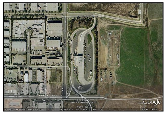
Trucks enter the southern end of the facility, and proceed along its western side through weigh scales. Vehicles and drivers that pass weight and credentials screening can exit the compound at its northwest corner onto northbound Enrico Fermi Drive. Vehicles that must undergo inspections are directed around the inspection facility in the center of the compound, and enter the covered inspection bays from the south. Once inspections are completed, vehicles can exit at the northeast corner of the compound onto Siempre Viva Road, either eastbound or westbound. Most vehicles head west from that exit.
Once the US bound crossing process is complete, trucks either complete their trip at one of the many warehouse facilities in the vicinity of the Otay crossing, or they continue west on Siempre Viva Road to Highway 905, which intersects with Interstate 805, Interstate 5, and Highway 125.
During the period of the test and data collection, the traffic volume at the Otay Mesa crossing dropped significantly from its daily average of 2,500 trucks. According to statistics provided by the CBP, the average daily volume ranged from just over 1,600 to approximately 2,000 trucks per day, with the average staying between 1,800 and 2,000 per day between June and November 2009. This reflects a drop of approximately 20 percent. The implication is that a smaller total number of trips by participating trucks would be required to meet the desired three to five percent of total truck trips.
3.2 Stakeholder Session Results
The stakeholder sessions offered valuable insights into the challenges faced by users and administrators at the border. They allowed for a much more comprehensive understanding of not only the conditions as they exist, but also regarding what might be done to improve them. While each stakeholder session was tailored to the specific groups represented, the general format for each session was as follows:
- Project Overview: the Study Team delivered basic project information summarizing the Otay Mesa test.
- Stakeholders were shown a live a Google Earth map to facilitate a discussion among participants to gain a "day in the life" overview of border workings from their perspective. The discussion was tailored to the stakeholder session attendees, and included a facilitated discussion of stakeholder observations regarding travel time through the Otay Mesa crossing, including:
- How often are delays experienced?
- Where do the delays occur (start and end)?
- Are there delays in both directions?
- Are there any patterns worth noting (e.g., changes based on days of week, other periods)?
- Stakeholders then took part in a facilitated discussion of border travel time information needs of the stakeholder group. This included summarizing the needs identified at Sessions 1 and 2 to state, local, and federal transportation agencies and customs representatives.
- The Study Team led a summary of the proposed technologies to be tested: GPS and ALPR.
- Stakeholders were then asked to look forward and offer thoughts on what the future holds for the crossing, including increases in trade traffic and how these may be related to information needs and/or any facility and technology programs planned or underway that might affect this project and potential future deployment.
- The sessions closed with a request for each stakeholder group to identify a representative to be part of a Technical Working Group. This group was to be utilized for any follow-up questions and/or to review proposed technologies or deployment locations.
In addition to the information presented in earlier sessions regarding the operations at the crossing, stakeholders provided some useful ideas regarding what would be a potential set of functional requirements for any border travel time measurement solution. These are provided in Table 2.
| Stakeholder Group | User Needs (Northbound) | Characteristics | Functional Requirements |
|---|---|---|---|
| FHWA | Measure a total cross border travel time from the beginning to the end of the queue; need historic data for planning applications | Without isolating any one agency, measure a cross-border travel time from beginning to end of queue | End of queue is likely the longest end point in peak season; measuring "too close" to the border will cause bias; travel times can be determined at two instrumented points, but load type may require additional analysis and/or another instrumented location |
| Motor Carriers | Real-time cross-border total travel time is of great interest for providing information to customers; GPS technology has implications for C-TPAT | Queues often back up to Calle 12 and Bellas Artes (peak season); queues usually reach the MX sorting gate; the exit of the CHP facility marks the end of the cross-border trip | Measure from the start of the queue at Calle 12 and Bellas Artes to a common point outside of CHP inspection, at the intersection of Enrico Fermi Drive and Siempre Viva Road; alternatively, measure at both CHP exit gates) |
| State and Local Transportation Agencies | For transportation systems operations, it is unlikely that historic or real-time data will affect procedures; however, any data of interest to customers will be incorporated into regional ITS | Real-time data will be utilized in the regional 511 system; data could be integrated into PeMS1 | Data requirements for PeMS integration will be explored; any data would be used and no one technology is preferred over another |
| US/MX Customs | Customs and Aduana are interested in intermediary measures; CBP notes that a measure of exiting MX gate through US primary is needed; must normalize for secondary inspections | Aduana is interested in measures from the beginning of the queue to/through MX customs; US CBP is interested in the total travel time and time to/through MX customs, but primarily in the time from exiting MX customs to/through US customs primary inspection |
Requires multiple measurement points; FAST, laden, and empty moves should be differentiated End of queue (1); MX sorting gate (2) to differentiate load type; entry to MX export lot (3); exit of MX export lot (4); entry to US primary (5); exit of US primary (6); common point outside of CHP facility (7 or 8) |
| 1 PeMS – California’s Freeway Performance Measurement System: The PeMS project is conducted and maintained by the University of California at Berkeley with cooperation from the California Department of Transportation (Caltrans), California Partners fro Advanced Transit and Highways, and Berkeley Transportation Systems. This statewide database collects historical and real-time freeway data from freeways in the State of California in order to compute freeway performance measures. | |||
3.3 Technology Selection
ALPR
Automatic license plate recognition is a specialized application of digital cameras to detect the presence of individual vehicles. License plate recognition is used for traffic management, weigh-in-motion commercial vehicle inspections, security, parking, and border control, as well as for toll collection and violation tracking. London's congestion pricing program, for example, uses license plate recognition to charge a fee to vehicles that enter central London during peak hours. Toronto's Highway 407 uses ALPR applications to toll system users whose vehicles are not equipped with radio frequency identification (RFID) toll transponders. The tolling system uses an ALPR system to capture vehicle license plate numbers. From there, optical character recognition (OCR) software is used to identify the plate numbers for billing the toll at a higher rate.7
ALPR-based travel time measurement systems work by electronically recording the front or rear license plates of vehicles as they pass mounted ALPR cameras or "out-stations." Once a vehicle passes an out-station, the system resolves the image into a string of alphanumeric characters and transmits the resulting string to an "in-station." This data transfer may happen via wired connection or wirelessly. After a vehicle passes two out-stations, the system then calculates the travel time between them.
ALPR technology is widely deployed in both the US and Mexico. ALPR vendors interviewed for this study also confirm the use of ALPR in Mexico for security applications. Intelligent Imaging Systems,8 for example, works closely with the City of Tijuana and states in the Mexican interior; Devices provided by imaging system supplier PIPS Technology are also widely deployed in Mexico. Both technologies can also detect license plates from various Mexican states.
ALPR applications for travel time measurement are not as widely deployed as the security and enforcement applications; however, ALPR can provide an accurate measurement of travel times between fixed locations provided that the cameras have an appropriate sight angle to read the license plates and that the license plates themselves are not too damaged or dirty for the camera to collect a "good read." ALPR can work both during the day and at night and is not dependent upon carrier participation. ALPR can theoretically collect data from the total vehicle population, up to the successful read rate. However, because an unimpeded visual line of sight to each plate is required to capture a complete image, sufficient space between commercial vehicles is needed. This may be a problem at congested border locations where nose-to-tail operations are common.9 Further, the security of ALPR infrastructure is of concern since roadway geometry and other factors may dictate that it must be mounted in areas outside of controlled-access facilities.
The most likely business model for deploying ALPR in Otay Mesa is to purchase ALPR equipment from an ALPR vendor and install two out-stations and one in-station to collect a total cross-border travel time. These installations would be located at the beginning and end of queue as detailed in the Task 1 Stakeholder Summary and would be permanent installations. Additional temporary installations could be utilized to collect a sample of information at various intermediate points. For example, such an installation would be necessary to capture data points at locations such as the exit of MX customs, the entrance to the US primary booths, or one for the FAST lanes entering US Customs. This temporary installation would then be used to collect representative sample of "average day" data that could be applied to extrapolate travel times by type of movement or between various points. This could be accomplished within the FHWA's budget for this study; however, funding for equipment maintenance and replacement past the equipment warranty, or to address vandalism would need to be identified and programmed for each installation.
GPS
GPS data are becoming more commonplace as a solution to collecting travel time information where fixed devices (including sensors and ALPR) cannot provide the same levels of area-wide coverage. Section 1201 of the Safe Accountable Flexible Transportation Equity Act – A Legacy for Users (SAFETEA-LU) has encouraged regional GPS deployments to collect traffic data. Section 1201 established the Real-Time System Management Information Program and encourages states to "monitor, in real-time, the traffic and travel conditions of the major highways" and to share data with local governments and travelers alike.10
Because of deployment, maintenance, and operations expenses associated with fixed travel time data collection technologies (such as loop detectors, fixed sensors, and even ALPR), GPS and other types of probe data (including cellular probe data) provide a cost-effective solution and can cover an entire metropolitan region.
Large-scale probe-based travel time data are currently being collected in Baltimore, MD; Missouri – statewide; San Francisco, CA; New York State; and at the northern border (among other locations nationwide). In Baltimore and Missouri, ITIS Holdings Plc. in partnership with Delcan is collecting probe data from the cellular phone network and from GPS-equipped commercial vehicles. In San Francisco, researchers at the University of California Berkeley have partnered with Nokia to test using GPS-enabled mobile phones to provide traffic information. Perhaps the largest GPS-based deployment to date is on the I-95 Corridor, from New Jersey to North Carolina, where INRIX was recently awarded a multi-year, multi-million dollar contract to provide travel time and speed data from more than 750,000 GPS-equipped vehicles.11
GPS-equipped vehicles are often used to calculate "ground truth" travel time estimates to evaluate the accuracy of travel times collected via fixed sensors. This technique is used to validate regional congestion information by the Baltimore Metropolitan Council, for example.12
GPS units can provide a continuous source of location information with an infinite number of measurement points; however, reporting cycles of equipment and vendors often dictate when a measurement is taken. Many carriers, for example, choose to have in-vehicle units send location information every 15 to 30 minutes as a means to manage the overall communications costs associated with such systems. Vendors transmitting location information on the cellular data network (Nextel, for example) may collect location information every 2-5 minutes.13 While older GPS units may not provide enough accuracy to detail lane-by-lane travel times, studies by the Institute of Transportation Engineers (ITE) and the Texas Transportation Institute (TTI) among others validate the accuracy of GPS-based traffic data.14
The FHWA is also engaged in GPS-based travel time measurement on a national scale. In work conducted under a project entitled "Freight Performance Measurement: Travel Time in Freight-Significant Corridors," the FHWA has been examining the use of GPS systems to calculate the average speed for trucks on specific road segments.15 The speeds of multiple trucks are then aggregated to determine average speed on a road segment. These measured speeds are then used to calculate travel time reliability along various routes. This same GPS data is being used to assess border crossing time at 15 US/Canada ports of entry.
At the Otay Mesa border, a number of different deployment options were considered for cross-border travel time measurement using GPS data. A key study objective was to utilize a deployment option and business model that could be sustained over time and have a high likelihood of adoption after the test was completed. These options are shown in more detail in Table 3, which discusses the characteristics of and the risks associated with each of four different deployment models.
| Deployment Model | Time to Implement | Historic Data Collection | Real-Time Data Collection | Contractual Agreements | Hardware | Software | Ownership | Future Operations | Cost | Risk |
|---|---|---|---|---|---|---|---|---|---|---|
| Collect GPS data by deploying units in trucks | 6 months for deployment followed by 1 year for data collection | Baseline data will be analyzed over time | Real-time data demonstration may require additional funding | Will require contracts with carriers; if carriers are paid for participation; contract oversight will be time-consuming and costly | Will require hard-mount GPS units in trucks; hand-held units may not provide accurate data, but could be considered | Will require basic algorithms to analyze data | FHWA will own baseline data and equipment after test conclusion | A continuation of this model is unlikely to be sustainable over time due to time spent facilitating arrangement with carriers and operations/ maintenance of equipment | Short-term costs are moderate, but carrier issues and project budget translate to high risk; additionally, long-term model not sustainable | High |
| Purchase GPS data from vendors (no carrier involvement) | 6-12 months for agreements followed by 1 year for data collection | Baseline data will be analyzed over time | Real-time data demonstration may require additional funding | Contracts with multiple vendors will be difficult to arrange; vendors may be unwilling to participate | No additional hardware; will use systems already deployed | Will require basic algorithms to analyze data | Baseline dataset will be public, but additional data use will require renegotiation with vendor | Likely to be sustainable over time if vendors are willing to participate; privacy concerns add risk | Short-term costs are moderate; risks are high due to privacy issues; better model involves carriers directly | High |
| Carrier request GPS data from vendor to be exported to Study Team | 6 months for data stream followed by 1 year for data collection | Baseline data will be analyzed over time | Real-time data demonstration may require additional funding | Will require contracts with carriers; if carriers are paid for participation; contract oversight will be time-consuming and costly | No additional hardware; will use systems already deployed | Will require basic algorithms to analyze data | Baseline dataset will be public, but additional data use will require renegotiation with carriers and vendors | Likely to be sustainable over time; however, maintaining contracts with carriers will be time consuming | Data collection costs are likely initially low, but may increase over time | Med |
| Collect travel time information from third-party provider (e.g. Calmar, Inrix) | 3-6 months for initial data stream, followed by 1 year of data collection | Baseline data will be analyzed over time | Real-time data demonstration may require additional funding | Will require agreement with third-party provider | No additional hardware; will use systems already deployed | No additional software for baseline data | Baseline dataset will be public, but additional data will require third-party provider | Sustainable- if third-party providers stay in business; cost may initially rise, then adjust to market conditions | Data collection costs are likely initially low for a "test;" provider may increase cost after test deployment | Low/Med |
The options for collecting GPS data from commercial vehicles crossing the international border at Otay Mesa are highlighted in Table 3 and summarized below. Because GPS equipment is largely a carrier-based asset, the business models must involve cross-border motor carriers in a way that is acceptable for their businesses. While the following deployment models are all potential methods of collecting GPS-based data, some make more sense than others in the case of the Otay Mesa deployment, where options with lower risk and greater likelihood of adoption are preferable.
Option 1: Deploy GPS units in trucks to collect baseline travel time data and validate technology. This would require purchasing GPS units and software to collect and aggregate these data as well as coordination with carriers for participation agreements. While this model is technically possible, its feasibility is doubtful. In addition to the expenses associated with device purchase and use, many larger carriers already have GPS-equipped vehicles and may be unwilling to participate. Additionally, the validity of the data may be in question, since the GPS equipment could be easily disconnected if it is deemed not valuable to business operations, if a driver feels it is intrusive, or if external parties become aware of its presence in vehicles. Government-owned GPS devices would also require FHWA-sponsored operations and maintenance, which would significantly complicate the contractual process. Table 3 summarizes this model as: Low feasibility, high risk.
Option 2: Purchase GPS data directly from vendors. Acquiring data directly from vendors provides a means to streamline GPS data collection. This method does not include purchasing any propriety information about the carriers themselves, only access to aggregated GPS data not segmented by carrier or carrier type. While some third-party providers have had success in purchasing data from GPS vendors, Delcan's experience in the US suggests that probe data that are provided from vendors or cellular phone carriers, while robust, are difficult to procure due to contracting and privacy issues. While carrier privacy would not be violated, carriers may perceive a privacy breach and question vendor rights in selling data. Table 3 summarizes this model as: Low feasibility, high risk for the purposes of this study; however, other initiatives may find success for this model with larger budgets and longer timeframes.
Option 3: Purchase GPS data directly from carriers and/or carriers request data feed from vendor. This business model will likely provide more success than working with the vendor. Three large carriers attending the Otay Mesa sessions have already agreed to provide GPS data for the test. These carriers, by agreeing to participate, would also likely share business characteristics (fleet size, FAST/CTPAT certified, empty movements, etc), which could be used to help statistically differentiate the travel times of the laden, FAST, and empty movements traversing the border. At the same time, contracting and data access issues will be more time consuming not only for the test, but for the FHWA over the long-term if the data stream is to be maintained. Finally, there is some concern that outside parties may not trust the data obtained directly from motor carriers, since carriers may be reticent to provide complete datasets directly to a government entity. Table 3 summarizes this model as: Medium feasibility, but high risk due to the high involvement of the FHWA in contracting with carriers.
Option 4: Purchase GPS data from a third party provider. Calmar Telematics and Inrix provide these services, among others. As third-party providers, they contract with the carriers and/or owners to collect GPS data either directly from the fleet's IT department or from the vendor. Fleets will ask vendors to push data to the third party provider, and the third party will then provide data for that specific carrier. Third party providers may pay between $20 and $100 per vehicle per year directly to the carriers. It should be noted that the payments are based on market conditions, where heavily congested urban areas often demand higher payments to carriers as third parties have more success reselling data in these areas. Calmar is currently providing data on the New York State Thruway and at the northern border Peace Bridge. Inrix was recently awarded a contract to provide data along the I-95 Corridor and provides data in cities nationwide.
To meet the project objectives, a GPS deployment strategy that utilizes a third-party provider (Option 4) was selected.
Acquiring GPS data from a third-party provider is not without risk, however, and data "ownership" issues must be addressed. The dissemination of raw GPS data is more likely to be restricted by the carrier or by the third party because of the issues associated with collecting, using and maintaining these data. In this case, the customer agency might have full rights to review the analyzed data and travel times and to disseminate summary information, but the raw data would likely have certain limitations for use outside of agency activities and may not be available directly to the agency. This was not a significant concern during the test, but may introduce more complex contracting language under deployed conditions.
Additionally, third-party providers may provide GPS data, which they purchase directly from motor carriers, for a greatly reduced cost for the purposes of the test. However, the cost of these data may increase (or decrease) based on coverage and market conditions. Delcan's experience with probe data shows that deployment costs may initially increase after the initial test period until they adjust for market conditions and/or a larger business to the third party is realized.16
Both GPS and ALPR were considered for deployment at Otay Mesa and were evaluated against the following User Requirements for technology deployment as detailed in the Task 1 Stakeholder Sessions. A summary comparison of ALPR and GPS for each User Requirement is shown in Table 4, with the primary User Requirements of:
- Total cross-border travel times (historic data);
- Total cross-border travel time with FAST, empty, and laden movements differentiated;
- Real-time information on delay; and
- Measures of travel times between multiple points within the US and MX Customs compounds.
It should be noted that not all user requirements could be addressed with this initial technology deployment; however, each technology and its potential to provide these capabilities was addressed in detail as shown in shown in Table 4.
| User Needs (Northbound) | GPS | ALPR |
|---|---|---|
| Total cross border travel time (historic) from the beginning to the end of the queue | GPS data can be used to provide a total cross-border measurement of travel times within FHWA's budget. GPS risks are related to carrier commitments to participate; however, carriers were eager to participate in the stakeholder session conducted in January 2008 and in follow-up contacts with stakeholders. | ALPR can be used to provide a total cross-border measurement of travel times within FHWA's budget. ALPR risks include safety and security of the ALPR equipment. The specific location of ALPR camera at beginning of queue has yet to be determined |
| Total cross-border travel time with FAST, laden, and empty moves differentiated | GPS data for each movement type may be differentiated using fleet characteristics and geo-fencing. This requires additional analysis and estimation using statistics. | Travel times will be estimated based on statistical distributions of trip types within the total sample. CBP crossing data, if provided, can enhance this analysis. |
| Real-time wait information: total travel time, FAST, laden, and empty | GPS data can be used to collect data on the approach to, as well as within, the customs compound and can provide real-time travel time information. | The total travel time using ALPR can be reported in real-time, but only after the truck passes both the first and last reader locations. |
| Travel time information between multiple points within the MX and US customs compounds | GPS data for multiple measurement points can be differentiated using geofencing, provided the location sampling frequency is high enough to capture a truck as it passes through a geofenced area (e.g., CBP secondary). This requires additional statistical analysis. | ALPR data for multiple measurement points can be collected using portable ALPR stations at temporary points. This requires additional analysis and estimation for segments not measured. Alternatively, could relate plate reads to CBP records showing crossings by individual trucks, if access to such data is permissible. |
| Data/ infrastructure ownership | GPS equipment will not be owned by the FHWA; raw GPS data may not be owned or even accessible to the FHWA. As a risk, carriers can choose to terminate data access at any time, but would lose revenue | FHWA will own both the infrastructure and the raw data, but will also be responsible for maintenance of the physical assets, which include at least two camera/antenna/power "out station" assemblies, and one "in station" to receive transmitted data. |
| Safety, security, and maintenance | No issues associated with safety and security – many GPS deployments by carriers support C-TPAT programs; however, maintenance of contracts with carriers is required. | Safety and security of ALPR infrastructure is primary concern. Life span of equipment is 3-5 years; more information is needed to assess useful life under rugged border conditions. Potential security risk from theft or damage to fixed infrastructure. |
| Long-term viability | Carrier commitments will likely change over time. For long-term viability, a third party can best address carrier contracts, where business models provide incentives to add more carriers and data-related service offerings. | Historical precedent exists regarding ability of agencies to support long-term maintenance, security, and life-span of equipment. Trends in state-of-practice suggest in the long-term, fixed infrastructure for travel time measurements will likely be replaced by probe technologies. |
| Stakeholder support | Stakeholders support sharing or selling of GPS data based on feedback obtained during January 2008 stakeholder sessions and follow-up phone calls/ emails. | Initial cost of infrastructure along with maintenance and security issues are sources of high stakeholder concern. Cameras near border may add additional privacy concerns for carriers. |
| Information beyond borders | Could potentially track trip origin, destination, and routes for more robust analysis. Could provide data for FHWA's freight travel time data base. Southbound data can be added at no additional deployment cost. | Could provide travel times with other ALPR sites from same vendor with additional software. Extension of geographic measurement window or addition of southbound data would require additional installations. |
Additionally, the following "other considerations" for deployment are documented in Table 4:
- Data and/or infrastructure ownership;
- Safety, security, and maintenance;
- Long-term viability of the technology;
- Stakeholder support for deployment; and
- Potential for a richer dataset "beyond" the border and/or on the southbound approach.
In summary, GPS data provide a robust stream of multiple data points. The continuous nature of the data allows for analysis of travel times for different segments of the cross border trip. Southbound information can also be added without additional deployment costs. The study team recommended a third-party provider approach to help mitigate risks from carrier involvement and data contracts; however, the provision of the data from the carriers was still the largest risk for GPS deployment. The January stakeholder sessions helped identify carriers who were willing to participate in this task. Stakeholders strongly supported GPS applications.
ALPR deployment can provide a concrete measure of the total cross-border travel time provided that the infrastructure can be mounted in a safe and secure location that is within range to read commercial license plates. Temporary ALPR stations can provide additional estimates of travel times for segments of the trip within the MX and US Customs compounds. Because the FHWA would be responsible for maintenance of ALPR infrastructure, safety and security is a significant risk.
3.4 Technology Deployment
Once the decision was made to go forward with a GPS-based deployment, data acquisition requirements were broadly described to the data provider. The key requirements were that the sample size be sufficient to provide the required volume of data to adequately characterize travel times and that carriers would need to allow unrestricted access to all available GPS data generated by trucks passing through the Otay Mesa crossing.
Prior research indicates that, in order to accurately characterize travel times on a roadway network, between three and five percent of the total vehicle population must provide GPS data on a regular basis.17 With a typical daily volume of 2,500 truck trips at the Otay crossing, this equates to between 75 and 125 truck trips daily.
In order to meet these requirements for truck GPS data, the data provider needed to identify and recruit motor carriers to participate in the project. The data provider's operating model involves the acquisition of GPS data directly from the carriers, as opposed to other vendors that obtain data from fleet management system providers. Though for business confidentiality reasons the data provider did not fully disclose the reasons for adopting this model, they did indicate a preference for dealing directly with the owners of the data, as opposed to negotiating agreements with system or service providers.
The data provider chose to address this requirement by recruiting three carriers with trucks that regularly travel the Otay crossing. Initially, the carriers were chosen because they already possessed vehicles with GPS data systems installed. This approach is taken for two primary reasons. First, because the carrier has ultimate ownership rights to the data, they can grant access directly, without requiring the approval of any additional party. Second, carriers are typically open to receiving modest compensation, since they incur no additional expense and can recoup a portion of their investment in fleet management systems and services.
The primary drawback of this approach is that individual agreements must be negotiated and maintained with each carrier. This proved especially challenging for this project. While the carriers from whom the data provider acquires GPS data are primarily US-based fleets-many that are located in the northeast US-many of those that use the Otay crossing are co-owned by families that have operations on both sides of the border. Hence, the nature of negotiations was somewhat unique, as compared to that which the data provider is accustomed. The result was that it took somewhat longer to negotiate agreements than might otherwise be required in a non-border environment.
Initial data received from the equipped trucks indicated that many of the trucks that appeared in the measurement zone did so only once or twice during a given trip, often on the Mexican side of the border before reaching US CBP primary inspection. This level of data was deemed by the team to be insufficient to reliably measure travel time in the Otay border zone.
Initially, the GPS data provided by the carriers that agreed to participate was generated with a trailer-tracking system called SkyBitz. While the position data provided by these systems has proven reliable over a number of years, it became clear as the test progressed that the reporting frequency was not sufficient for measuring travel time over such a short distance. Skybitz systems typically report position every 30 minutes, plus provide additional reports when vehicles begin moving, or stop for a predetermined period of time.
Because the existing carrier agreements with SkyBitz did not generate data with enough frequency to provide a sufficient number of data points within the border travel time measurement zone, and because the participating carriers often move trailers that are not equipped with SkyBitz devices, To address this, the participating carriers opted to upgrade their GPS units. These units, provided by LocJack, are designed to be installed in the tractor. The units capture position data every two to three minutes, and forward reports within 10 minutes. Going this route meant that the opportunity existed to also capture the movement of unequipped trailers and bobtail trucks (trucks without trailers attached).
Carriers utilized the compensation provided to them through their data agreement with the data provider to purchase and install a total of 175 units in trucks. The devices were installed and brought on line during the February to April timeframe in 2009. The carriers purchased these units at a price of $350 per unit, and subscribed to data services at a cost of $17 per month. Once the units were installed, the data provider was granted access to data feeds by the carriers.
While the study team was not a party to the specific terms and conditions of the agreements between the data provider and the carriers, the terms included a provision to provide anonymous data to the study team, and by extension to the FHWA, for all US-bound truck trips occurring within the area in the immediate vicinity of the crossing, and all data points falling within the measurement zone, for a period of one year. This was agreed upon by the carriers in return for the provision of data from the GPS units.
3.5 Trip Statistics
As previously discussed, the average daily truck traffic volume at the beginning of the test was expected to be approximately 2,500 trips per day. Using the general rule of thumb that between three and five percent of the vehicle total needs to provide probe data in order to accurately characterize travel times, this places the desired number of daily trips by equipped vehicles between 75 and 125.
In actuality, during the test the total vehicle counts were consistently lower than the 2,500 figure. CBP provided data that indicated that the average daily US-bound vehicle count. Table 5 shows the total (including loaded and empty) truck counts by month, plus the daily averages for the period from January 2009 through February 2010.
| Month | Total Truck Counts | Daily* Truck Counts | Loaded Truck Counts | Empty Truck Counts |
|---|---|---|---|---|
| Jan-09 | 51,766 | 1,922 | 31,787 | 20,099 |
| Feb-09 | 48,205 | 2,040 | 30,501 | 18,465 |
| Mar-09 | 55,285 | 2,126 | 35,758 | 19,527 |
| Apr-09 | 56,709 | 2,181 | 37,242 | 19,467 |
| May-09 | 54,790 | 2,107 | 36,778 | 18,012 |
| Jun-09 | 60,191 | 2,314 | 38,851 | 21,321 |
| Jul-09 | 60,550 | 2,047 | 39,560 | 21,862 |
| Aug-09 | 57,821 | 2,224 | 36,682 | 21,141 |
| Sep-09 | 59,743 | 2,298 | 39,094 | 20,649 |
| Oct-09 | 64,848 | 2,402 | 43,236 | 21,612 |
| Nov-09 | 58,879 | 2,355 | 39,545 | 19,334 |
| Dec-09 | 55,638 | 2,059 | 37,207 | 18,389 |
| Jan-10 | 51,020 | 1,962 | 32,504 | 18,516 |
| Feb-10 | 50,816 | 2,201 | 33,884 | 18,945 |
| * Based on Mon-Sat. Sundays were excluded because trip counts are very small. | ||||
According to port officials at Otay Mesa, approximately one third of the total laden shipments are FAST trips.
In order to assess whether the fleets participating in the project were providing an adequate percentage of overall trips, the study team examined the GPS data to identify two different types of trips. The first was "total trips." For this category, any appearance of multiple points from the same truck within the dataset for a given two-hour period was considered a trip. This was true regardless of where the points were located, as long as they were within the travel time measurement zone, and indicated US-bound movement. The second trip type was "crossed trips." The study team considered a trip a crossed trip if a truck reported its position at least once on each side of the border during an individual trip. Hence, the group of total trips included all crossed trips, plus any additional trips for which points could not be identified on one side of the border or the other.
Figure 8 contains a plot of the data gathered during the test from January 2009 through March 2010. It illustrates the number of trips for which data was captured during each month. The acronym MOY represents month of the year.
Figure 8. Otay Mesa Data Trips – January 2009 through March 2010
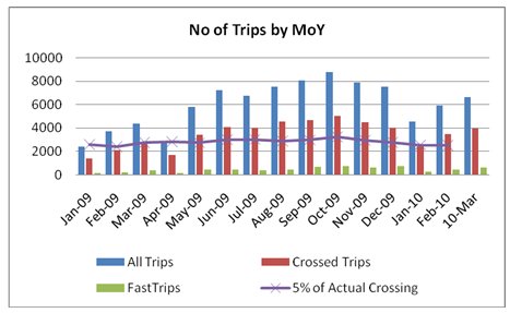
As the data indicate, the number of crossed trips for which GPS data was collected consistently fell between three and five percent of the total trips through the border as reported by CBP.18 Based on these figures, the study team was confident it could rely upon the data from crossed trips to characterize travel time through the crossing. The alternative would have been to attempt to construct composite travel times from the totality of the captured trips. The team considered this unnecessary and therefore did not attempt it.
As the graph shows, the number of trips that the team was able to identify as FAST trips was very small. The FAST trips generally equated to between 10 and 18 percent of the total crossed trips on a monthly basis, with just under 13 percent over the duration of data collection. The team arrived at these figures by creating a "geofence"19 around the portions of the MX customs compound through which only FAST trucks travel. This was accomplished using TransCAD, overlaying all of the points on the map grid for the crossing, and identifying individual truck GPS data points that fell within the area. A graphical depiction of this geofenced area is provided in Figure 9.
Figure 9. Illustration of Geofence Used to Identify FAST Trips
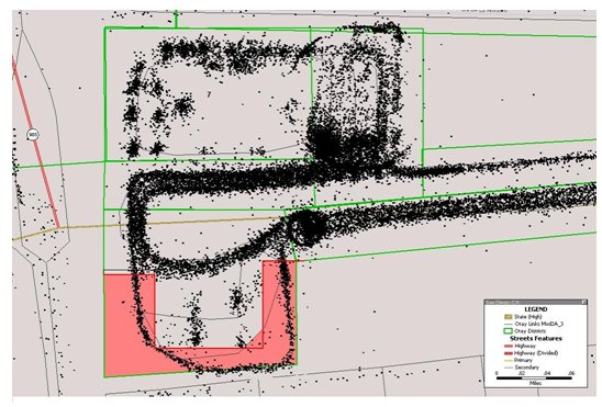
The study team designated the area indicated in red as the most likely opportunity to isolate trucks completing FAST trips. The small black dots superimposed over the image represent individual GPS data points received from participating trucks. As the image indicates, there is a distinct separation in traffic flow. However, based upon the figures cited by the carriers regarding the percentage of trips conducted as FAST trips, the method clearly resulted in under-reporting.
By contrast, the study team was confident that the method was appropriate for the identification of vehicles that passed through secondary inspection, which includes the screening of vehicles by x-ray units on the western end of the US customs compound. Vehicles directed to secondary for x-ray screening pass along the upper perimeter of the compound from east to west, then turn south to pass through one of two x-ray units. Travel speeds are typically low through this area, and every truck must come to a stop during the x-ray screening process. The result is that vehicles directed to complete this screening can be expected to report multiple times while in secondary.
The team also analyzed crossing data by day of the week (DOW) and time of day (TOD). Figures 10 and 11 illustrate the distribution of trips for these parameters.
Figure 10. Otay Mesa Data Trips by Day of the Week
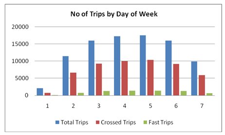
In Figure 10, the days of the week start with Sunday, which is designated as day 1, and end with Saturday, which is day 7. As the data indicate, Wednesdays and Thursdays were the busiest days, while very little traffic crossed on Sundays. With the exception of Sundays, the number of crossed trips captured for each day type was consistently above 500, with values approaching or exceeding 1000 trips for all days from Tuesday through Friday.
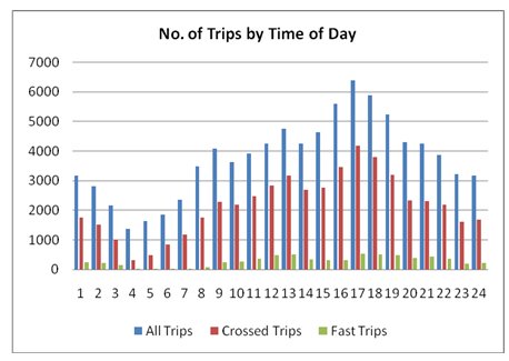
The data illustrated in Figure 11 requires more explanation. The crossing itself is closed between midnight and 8 AM. However, there are two phenomena that result in the appearance of trips during those hours. The first is that trips that begin late at night, and include processing through US customs primary prior to the midnight closure must still complete the trip through customs and the CHP inspection facility. This phenomenon likely accounts for most of the trips reported until the 4 AM low point. The second phenomenon, which likely accounts for most of the trips between 5 and 8 AM, is the queuing of trucks awaiting the opening of the border. In any case, the data for the period from 3 AM up until 6 AM is very sparse, and are not considered reliable.
Figure 11. Otay Mesa Data Trips by Time of Day
3.6 Border Travel Time Data
The accumulation and processing of individual GPS data points is a multi-step process. GPS data from the units used during this test is similar to data that would be forwarded from other GPS devices. The units transmit numerical values for latitude and longitude, along with a time stamp (in Greenwich Mean Time – GMT) and a unit identifier. Each of these points is then translated into a position on a roadway grid (see Figure 9 above), along with a direction of travel, and from that data vehicle speed and travel time can be calculated.
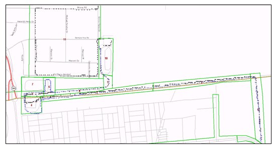
For this project, both the data provider and the study team ran calculations on the data, with the data provider conducting initial filtering and mapping, the forwarding it to the study team for analytical computation. At the onset of the data collection effort, the data provider created a set of geo-registered spaces that represented segments of the trip through the Otay crossing. These spaces, which are referred to as "districts," are shown as segments outlined in green polygons in the illustration in Figure 12, which also contains data from one empty vehicle trip through the border (dark blue dots) and one FAST truck trip (light blue dots).
The purpose of this was to allow for the consideration of partial trips in the overall calculation of travel time through the measurement zone. It was initially intended to accommodate the infrequent reporting intervals of the Skybitz devices. When the LocJack devices were brought on line, these districts simply became convenient mechanisms for observing partial-trip travel times, and to identify whether trucks were completing FAST trips or were unloaded.
Figure 12. Sample Otay Mesa GPS Data in Districts
For the purposes of understanding the translation of individual GPS points into travel time calculation parameters, it is useful to review the data manipulation sequence used during the project. The following sequence of actions took place for the data captured during the test:
Data Processing Sequence
- Data is collected from units:
- If the carrier has a database, Calmar applies a tool (created by them) that polls the carrier database, translates the GPS data into XML20 format, and then sends it to Calmar using encrypted TCP/IP.21
- If a carrier uses the provider website (rather than its own database), Calmar accesses the XML or .csv22 feeds through the website with a tool they created
- GPS data is fed into a "threshold database," which contains all raw data
- Calmar applies routines to process the GPS data and store in a "national database."
- Assigns a token ID to each GPS point.
- Strips specific vehicle identifiers, replacing them with a weeklong artificial identifier
- Snaps individual GPS points to the roadway grid using a routine written by Calmar,23 and the Navteq database shape file
- Snapping results – the results of the snapping routine are rows in a database file with the following headings
- roadID – node to node breakdowns
- linkNum – segment of road
- DistToSeg-Ft – perpendicular distance from an individual GPS point to roadway segment
- DistFrom_Ft – distance from projected point (point location on link) to beginning of segment
- Method – internal reference identifier that helps to sort dataset and understand characteristics of subsets of the dataset
- Labels are applied to different SensorStatus points (also labeled as "Reason"), based on what is and isn't known (start, stop, breadcrumb,24 etc.)
- GPS data is picked from the database using a specific area of interest defined as a box defined by lat/long corner points. For this project, this is defined as a rectangular area that fully encompasses all of the roadway segments that constitute the measurement zone.
- Outliers are identified and excluded by analyzing for unreasonable speeds between successive points.
- GPS data is fed into a GIS25 where it is associated with a selected area or district bounded by a geo-registered space. Then a geospatial overlay is superimposed over the dataset to bind the area/district identifier to the GPS data.
- A series of geospatial transforms is applied:
- The district of interest in which an individual point resides is associated with the underlying link structure as well as the GPS – i.e., a district ID is assigned. If the point is not in a district, the district identifier is a null.
- Export GIS data that has been snapped to a district of interest into a statistical analysis package.26
- Within the statistical analysis package, data parsing modifies the dataset to add useful characteristics (e.g., day of week, month, etc.), and to sort by different criteria.
- The system then tries to identify logical trip chain endpoints using elapsed time between consecutive points from an individual vehicle. Elapsed time clock (time between consecutive GPS points from the same vehicle) is reset to zero when a vehicle reappears in the dataset after having been absent for more than 6-1/2 hours.
- Single points are tossed out if there is not another data point within the districts within the 6-1/2 hour window.
- The refined output is placed into a data file to facilitate the calculation of travel times.
Many of the individual actions within this sequence required manual triggering of calculations or processing. As such, it is not likely to be useful for anything other than examination of data after the fact.
For the purposes of analyzing the data generated during the test, the study team fed the data into Excel and compiled statistical summaries of travel time. Because the travel time measurement zone was defined as the full distance between the Bellas Artes/Calle Doce intersection to the exit of the CHP facility (see Figures 3 and 4), the travel times were initially calculated to reflect that distance.
As described above, to facilitate calculating travel time across the full measurement zone and for portions of the trip, the trip length was segregated into a series of consecutive travel zones, or districts. The data provider formulated a set of eleven travel districts and provided the GIS shapefile to the study team for use during data collection and analysis. The image in Figure 13 shows all of the districts.
Figure 13. Otay Mesa Travel Time Measurement Districts
This was initially done to accommodate the compilation of travel time using portions of trips as reported by vehicles using the Skybitz solution, which, as was indicated previously, reports relatively infrequently. Ultimately, this became unnecessary. However, the districts were still utilized for determining the portion of the total trip travel time that was accumulated on the approach to the US customs primary inspection facility.
Based on the original definition of the measurement zone, the travel time calculation consisted of the total time elapsed between the first appearance of a truck GPS data report within district 1 and the last report within district 10. Using this approach, the study team concluded that there was a risk that the calculated travel time would be underreported, since conceptually speaking, a truck GPS unit could travel two to three minutes into the trip before issuing an initial report, and could then issue its last report two to three minutes before leaving the measurement zone on the US side. Ultimately, the team concluded that little could be done to correct for this and that given the typical travel times calculated, it would have a minimal effect.
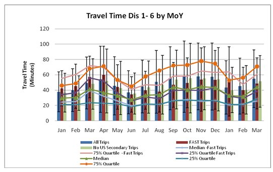
The charts in Figures 14, 15, and 16 show the calculated border travel time values for the trips observed during the test period, by day of the week, month of the year, and time of day. In each of the figures, travel time is presented in seconds, and the data is segregated to show all trips, and FAST trips.
Figure 14. Calculated Travel Time Values by Day of the Week (Dist 1 – 10)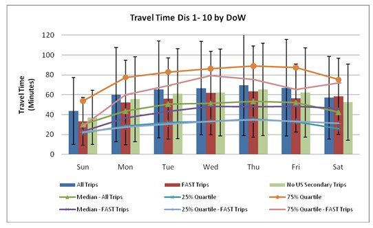
The vertical red, blue and green bars indicate mean travel time for all crossed trips, all FAST trips, and all trips for which the truck did not pass through secondary inspection, respectively. The vertical black interval lines represent the calculated standard deviation values for each mean value. The green line with intervals designated by triangles represents the median travel time for all trips, and the purple line with intervals designated by x's represents the median travel time value for FAST trips. Finally, the remaining lines represent the 25% and 75% quartile values for all trips and FAST trips.
The values presented in Figure 14 indicate that the mean measured travel time across the entire measurement zone for Mondays through Saturdays was between 60 and 70 minutes. Sundays, which as stated previously see very limited traffic, showed a mean travel time value of approximately 43 minutes. The data suggests that average travel times are longest on Thursdays and Fridays. The data corresponding to Figure 14 is provided in Table 6, which shows mean border travel time values and standard deviation values by day of the week.
| Day of Week | All Trips | FAST Trips | Non-Secondary Trips | ||||
|---|---|---|---|---|---|---|---|
| Mean Travel Time 1-10 | Stdev | Mean Travel Time 1-10 | Stdev | Mean Travel Time 1-10 | Stdev | ||
| Day 1 | Sun | 44 | 34 | 33 | 24 | 37 | 27 |
| Day 2 | Mon | 60 | 47 | 52 | 43 | 55 | 43 |
| Day 3 | Tue | 65 | 49 | 56 | 41 | 61 | 45 |
| Day 4 | Wed | 67 | 47 | 62 | 42 | 62 | 44 |
| Day 5 | Thu | 70 | 51 | 63 | 46 | 65 | 47 |
| Day 6 | Fri | 67 | 48 | 57 | 34 | 62 | 45 |
| Day 7 | Sat | 57 | 42 | 58 | 38 | 52 | 38 |
One notable characteristic in the dataset is that FAST trips-at least those that could be identified definitively-take less time for all days except Saturdays. Differences range from values of 15 percent lower on Mondays for FAST trips to just over 10 percent lower on Thursdays. This does not include Sundays, where differences are negligible and crossing numbers are very low. Saturday data suggests that FAST trips take an average of 2 percent longer. However, given the low level of confidence associated with the identification of FAST trips using the GPS data, this value cannot be considered significant.
Also notable within the data is the very large value associated with the standard deviation from the mean. The values calculated from the data indicate that the standard deviation ranged from 61 percent to 81 percent of the mean. These values suggest that the carriers that participated in the study experienced very wide fluctuations in travel times.
Because the standard deviation values were so high, the study team was concerned that a small number of trips with inordinately high or low travel times were potentially influencing the values to a high degree. This is not uncommon for datasets where the sample is non-random, and where there are extenuating circumstances that may influence the outcome, such as variability in enforcement methods. In the case of travel times, vehicles that are delayed for extended periods, or that queue in advance of the opening of the border, may influence the data to such an extent that the mean values are biased to the high side. Because it is less prone to the influence of outliers, the study team also calculated median travel time values for each day of the week. As Figure 13 shows, the median values were measurably lower than the mean values. The data indicated that the median values were 15 to 30 percent lower than the mean values, which would place the median travel time for Mondays through Saturdays between 42 and 53 minutes.
The upward bias in mean travel time values is revealed further through the identification of 25% and 75% quartile values. These values form the upper and lower limits of observed travel times for the middle 50% of all observed trips. A comparison of the portions of the standard deviation range outside the middle 50% to those inside reveals that more of the deviation interval lies to the upper side of the range.
Figure 15 shows similar values for the crossing by month of the year between January 2009 and March 2010.
Figure 15. Calculated Travel Time Values by Month of the Year (Dist 1 – 10)
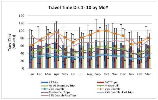
The travel time data characteristics for the months shown in the figure are consistent with those in Figure 14, with a few notable unique characteristics and observable differences. The first notable characteristic is that the mean and median travel time values peaked in the March-April 2009 and September-October 2009 timeframes.
According to CBP crossing statistics, the September-October 2009 period was the busiest period (see Table 5). This would seem to correlate with the increases in mean and median travel times. Interestingly, this is not the case with the March-April peak travel time values. The CBP crossing volume data indicates that the June-July 2009 timeframe was busier than the March-April 2009 time period. Unfortunately this is not explainable directly from the data.
The monthly data also indicates that the mean travel times for FAST trips were lower than the overall average for all but three of the months: January 2009, April 2009, and January 2010. Finally, the monthly data is consistent with the daily data in that they show that the median travel time is consistently lower than the mean, and that the middle 50% of trips fall to the lower end of the standard deviation range. Table 7 contains a summary of the mean and standard deviation values by month.
 |
Month and Year | All Trips | FAST Trips | No US Secondary Trips | |||
|---|---|---|---|---|---|---|---|
| Mean Travel Time 1-10 | Stdev | Mean Travel Time 1-10 | Stdev | Mean Travel Time 1-10 | Stdev | ||
| Month 1 | Jan-09 | 60 | 43 | 62 | 32 | 55 | 39 |
| Month 2 | Feb-09 | 62 | 49 | 60 | 34 | 59 | 47 |
| Month 3 | Mar-09 | 68 | 43 | 65 | 28 | 62 | 39 |
| Month 4 | Apr-09 | 69 | 50 | 79 | 58 | 63 | 45 |
| Month 5 | May-09 | 63 | 45 | 54 | 35 | 61 | 43 |
| Month 6 | Jun-09 | 54 | 39 | 53 | 35 | 50 | 37 |
| Month 7 | Jul-09 | 63 | 46 | 54 | 42 | 60 | 42 |
| Month 8 | Aug-09 | 67 | 48 | 54 | 39 | 62 | 46 |
| Month 9 | Sep-09 | 75 | 55 | 58 | 38 | 71 | 50 |
| Month 10 | Oct-09 | 76 | 56 | 61 | 39 | 72 | 53 |
| Month 11 | Nov-09 | 70 | 50 | 62 | 44 | 66 | 45 |
| Month 12 | Dec-09 | 68 | 48 | 62 | 41 | 62 | 45 |
| Month 13 | Jan-09 | 53 | 42 | 59 | 46 | 48 | 41 |
| Month 14 | 10-Feb | 54 | 42 | 49 | 35 | 48 | 36 |
| Month 15 | 10-Mar | 65 | 46 | 61 | 47 | 60 | 41 |
Finally, Figure 16 illustrates the travel time data broken out by time of day.
Figure 16. Calculated Travel Time Values by Time of Day (Dist 1 – 10)
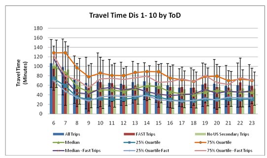
The time of day (TOD) dataset reflects the total travel time experienced by vehicles based upon the hour of the day when they first appeared in the system. For example, the value shown for hour 19 indicates that the mean travel time is approximately 62 minutes for trucks that first entered the measurement zone at 7 PM local time.
The more notable characteristics of the TOD dataset are as follows. First, because the number of points was exceedingly small, all trips identified as having started between 12 AM (when the border closes) and 6 AM were excluded from the dataset. The study team did this because it did not have confidence in the values provided. Second because the border does not open until 8 AM local time, the high travel time values reported between 6 AM and the opening of the border suggest that some vehicles are queuing in advance in order to ensure earlier entry into the US.
This would explain why travel times are longer for those vehicles, despite the fact that lower numbers of vehicles are processed in the early hours than in the peak volume hours between 4 PM and 7 PM (see Figure 11). Interestingly, the increase in volume seen in the peak afternoon/evening travel period does not translate into longer travel times. This is likely due at least in part to higher staffing levels during those periods.
Table 8 contains a summary of the mean and standard deviation values by time of day.
As was indicated previously, the travel time values presented to this point included the entire trip through the measurement zone from the Bellas Artes/Calle Doce intersection all the way through the exit of the CHP inspection facility. The study team and FHWA selected this as the measurement zone because it reflects the total border crossing as experienced by the truckers. While this is likely to be the most useful measurement zone, the nature of the GPS data suggests that it may be useful for the examination of portions of the trip, as well. This might be useful to isolate factors that may contribute to overall travel time, such as infrastructure geometry and overall facility capacity.
|
Time | All Trips | FAST Trips | No US Secondary Trips | |||
|---|---|---|---|---|---|---|---|
| Mean Travel Time 1-10 | Stdev | Mean Travel Time 1-10 | Stdev | Mean Travel Time 1-10 | Stdev | ||
| Hour 0 | 12:00 AM | 60 | 48 | 56 | 36 | 53 | 39 |
| Hour 1 | 1:00 AM | 53 | 32 | 43 | 30 | 47 | 26 |
| Hour 2 | 2:00 AM | 48 | 38 | 41 | 24 | 45 | 37 |
| Hour 3 | 3:00 AM | 87 | 0 | 97 | 0 | 81 | 64 |
| Hour 4 | 4:00 AM | 123 | 0 | 35 | 0 | 123 | 65 |
| Hour 5 | 5:00 AM | 124 | 0 | 96 | 0 | 120 | 52 |
| Hour 6 | 6:00 AM | 106 | 50 | 85 | 46 | 105 | 50 |
| Hour 7 | 7:00 AM | 99 | 59 | 60 | 67 | 93 | 49 |
| Hour 8 | 8:00 AM | 72 | 50 | 54 | 45 | 69 | 48 |
| Hour 9 | 9:00 AM | 65 | 55 | 67 | 48 | 59 | 47 |
| Hour 10 | 10:00 AM | 71 | 58 | 64 | 52 | 62 | 51 |
| Hour 11 | 11:00 AM | 65 | 49 | 61 | 38 | 60 | 46 |
| Hour 12 | 12:00 PM | 63 | 45 | 59 | 35 | 58 | 41 |
| Hour 13 | 1:00 PM | 67 | 44 | 59 | 30 | 63 | 43 |
| Hour 14 | 2:00 PM | 69 | 39 | 59 | 31 | 66 | 36 |
| Hour 15 | 3:00 PM | 67 | 43 | 57 | 45 | 65 | 42 |
| Hour 16 | 4:00 PM | 60 | 46 | 56 | 44 | 57 | 46 |
| Hour 17 | 5:00 PM | 55 | 40 | 56 | 42 | 52 | 39 |
| Hour 18 | 6:00 PM | 55 | 42 | 55 | 37 | 50 | 38 |
| Hour 19 | 7:00 PM | 61 | 46 | 64 | 41 | 57 | 40 |
| Hour 20 | 8:00 PM | 63 | 51 | 57 | 47 | 56 | 43 |
| Hour 21 | 9:00 PM | 59 | 44 | 55 | 36 | 52 | 37 |
| Hour 22 | 10:00 PM | 60 | 46 | 66 | 51 | 54 | 39 |
| Hour 23 | 11:00 PM | 59 | 44 | 49 | 37 | 53 | 35 |
In order to examine the efficacy of partial trip travel time measurement, the study team also analyzed the data to calculate the travel time from the beginning of the measurement zone to the exit from the US Customs primary inspection facility. This facility is represented as zone 6 in the dataset (see Figure 11). Hence, the travel time for this measurement zone would include the time elapsed between the first time a vehicle reported in zone 1 through the last time it reported in zone 6. The result of this analysis is illustrated in Figures 17 through 19.
Figure 17. Calculated Travel Time Values by Day of the Week (Dist 1 – 6)The most immediately identifiable characteristic is that the mean and median travel time values for the district 1 – 6 dataset are consistently approximately 75 to 80 percent of the district 1 – 10 values. This indicates that approximately three-quarters of the total travel time is spent queuing for and processing through US Customs primary inspection. The second notable characteristic is that the standard deviation is a slightly higher percentage of the mean, averaging from three to ten percentage points higher than those for the district 1 – 10 values. This suggests that travel time variability is more dependent upon the portion of the trip between the beginning of the measurement zone and the exit of the US compound than those portions afterwards. This is a reasonable result given the variety of screening actions that may be taken by CBP.
The data corresponding to Figure 17 is provided in Table 9, which shows mean border travel time values and standard deviation values by day of the week.
| Day of Week | All Trips | FAST Trips | Non-Secondary Trips | ||||
|---|---|---|---|---|---|---|---|
| Mean Travel Time 1-6 | Stdev | Mean Travel Time 1-6 | Stdev | Mean Travel Time 1-6 | Stdev | ||
| Day 1 | Sun | 23 | 20 | 33 | 24 | 30 | 25 |
| Day 2 | Mon | 45 | 37 | 37 | 31 | 42 | 35 |
| Day 3 | Tue | 52 | 40 | 47 | 35 | 49 | 37 |
| Day 4 | Wed | 52 | 40 | 48 | 34 | 49 | 38 |
| Day 5 | Thu | 54 | 41 | 49 | 32 | 52 | 39 |
| Day 6 | Fri | 52 | 39 | 48 | 32 | 48 | 37 |
| Day 7 | Sat | 46 | 37 | 55 | 38 | 43 | 33 |
The data shown in Figure 18 indicates these findings are consistent when the travel times are examined by month of the year.
Figure 18. Calculated Travel Time Values by Month of the Year (Dist 1 – 6)
The data corresponding to Figure 18 is provided in Table 10, which shows mean border travel time values and standard deviation values by day of the week.
The data shown in Figure 19 indicates these findings are consistent when the travel times are examined by time of day.
|
Day of Week | All Trips | FAST Trips | No US Secondary Trips | |||
|---|---|---|---|---|---|---|---|
| Mean Travel Time 1-10 | Stdev | Mean Travel Time 1-10 | Stdev | Mean Travel Time 1-10 | Stdev | ||
| Month 1 | Jan-09 | 60 | 43 | 62 | 32 | 55 | 39 |
| Month 2 | Feb-09 | 62 | 49 | 60 | 34 | 59 | 47 |
| Month 3 | Mar-09 | 68 | 43 | 65 | 28 | 62 | 39 |
| Month 4 | Apr-09 | 69 | 50 | 79 | 58 | 63 | 45 |
| Month 5 | May-09 | 63 | 45 | 54 | 35 | 61 | 43 |
| Month 6 | Jun-09 | 54 | 39 | 53 | 35 | 50 | 37 |
| Month 7 | Jul-09 | 63 | 46 | 54 | 42 | 60 | 42 |
| Month 8 | Aug-09 | 67 | 48 | 54 | 39 | 62 | 46 |
| Month 9 | Sep-09 | 75 | 55 | 58 | 38 | 71 | 50 |
| Month 10 | Oct-09 | 76 | 56 | 61 | 39 | 72 | 53 |
| Month 11 | Nov-09 | 70 | 50 | 62 | 44 | 66 | 45 |
| Month 12 | Dec-09 | 68 | 48 | 62 | 41 | 62 | 45 |
| Month 13 | Jan-09 | 53 | 42 | 59 | 46 | 48 | 41 |
| Month 14 | 10-Feb | 54 | 42 | 49 | 35 | 48 | 36 |
| Month 15 | 10-Mar | 65 | 46 | 61 | 47 | 60 | 41 |
Figure 19. Calculated Travel Time Values by Time of Day (Dist 1 – 6)
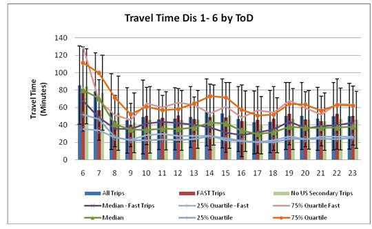
The data corresponding to Figure 19 is provided in Table 11, which shows mean border travel time values and standard deviation values by day of the week.
|
Time | All Trips | FAST Trips | No US Secondary Trips | |||
|---|---|---|---|---|---|---|---|
| Mean Travel Time 1-6 | Stdev | Mean Travel Time 1-6 | Stdev | Mean Travel Time 1-6 | Stdev | ||
| Hour 0 | 12:00 AM | 46 | 35 | 43 | 28 | 42 | 31 |
| Hour 1 | 1:00 AM | 44 | 31 | 47 | 29 | 41 | 28 |
| Hour 2 | 2:00 AM | 38 | 31 | 36 | 24 | 35 | 29 |
| Hour 3 | 3:00 AM | 64 | 0 | 30 | 0 | 66 | 64 |
| Hour 4 | 4:00 AM | 108 | 0 | 61 | 0 | 110 | 59 |
| Hour 5 | 5:00 AM | 99 | 0 | 44 | 0 | 97 | 50 |
| Hour 6 | 6:00 AM | 86 | 45 | 81 | 49 | 84 | 43 |
| Hour 7 | 7:00 AM | 79 | 44 | 57 | 35 | 77 | 43 |
| Hour 8 | 8:00 AM | 55 | 43 | 45 | 30 | 54 | 43 |
| Hour 9 | 9:00 AM | 45 | 38 | 40 | 25 | 42 | 34 |
| Hour 10 | 10:00 AM | 49 | 43 | 50 | 33 | 46 | 38 |
| Hour 11 | 11:00 AM | 46 | 34 | 48 | 36 | 45 | 33 |
| Hour 12 | 12:00 PM | 47 | 36 | 51 | 30 | 45 | 34 |
| Hour 13 | 1:00 PM | 49 | 35 | 47 | 25 | 46 | 33 |
| Hour 14 | 2:00 PM | 54 | 39 | 49 | 38 | 51 | 35 |
| Hour 15 | 3:00 PM | 53 | 40 | 49 | 40 | 51 | 38 |
| Hour 16 | 4:00 PM | 47 | 37 | 45 | 41 | 44 | 35 |
| Hour 17 | 5:00 PM | 43 | 36 | 46 | 38 | 40 | 33 |
| Hour 18 | 6:00 PM | 44 | 36 | 47 | 37 | 40 | 32 |
| Hour 19 | 7:00 PM | 50 | 39 | 53 | 36 | 47 | 35 |
| Hour 20 | 8:00 PM | 50 | 38 | 46 | 32 | 46 | 34 |
| Hour 21 | 9:00 PM | 47 | 36 | 45 | 39 | 44 | 33 |
| Hour 22 | 10:00 PM | 40 | 39 | 53 | 40 | 47 | 36 |
| Hour 23 | 11:00 PM | 50 | 38 | 51 | 34 | 46 | 33 |
The root cause of the high degree of travel time variability is not known for certain. However, the study team suspects that several factors may contribute to it. Fluctuations in demand volume, the opening and closing of primary screening lanes, the proportion of trucks participating in the FAST expedited screening program, variations in screening actions undertaken by US CBP can affect travel time. For example, during the team members' visit to the crossing, they observed an operation termed "blocking" by CBP staff. In this operation, trucks that have passed through the US Customs primary inspection booth are directed to form several northbound lines inside the compound, and are held stationary until the lines are filled. Once the lines are filled, CBP staff performs canine screening of all of the stationary trucks by walking around all of the trucks. Once the screening is complete the trucks are released in unison, whereupon they complete the u-turn to head south back through the exit of the compound and proceed on to the CHP inspection facility.
This activity is conducted on a periodic basis, at different times, and for obvious reasons is not announced in advance. Hence, while initial screening at the primary inspection booth may take no more than a minute, the trucks that are subjected to blocking are likely to encounter travel time increases of five to fifteen minutes, depending upon their position in line and the speed with which the canine screening can be completed. Given a mean travel time in the 60-minute range, such activities could easily result in measurable variations.
In order to gain a more complete perspective on the characteristics of the data set-and more importantly, develop a better understanding of the effects of outliers on the mean and median travel times-the team examined the frequency of occurrence of travel times within various "bands" or ranges. The results of this analysis are illuminating, and could have a significant effect on the methodology that should be applied when analyzing travel time data, particularly under near real time conditions.
The graph in Figure 20 depicts the cumulative distribution of travel times for trips from district 1 through district 10. As the image shows, 90 percent of all trips incurred a travel time of less than 133 minutes, and 90 percent of FAST trips took less than 100 minutes to complete. Figure 21 offers a slightly different view of the same data. It depicts the distribution of individual trips across the measurement zone by range of travel time.
These results suggest that is may be advantageous to examine the use of an arithmetic filtering process by which the trips with the longest travel times are removed from mean and median travel time calculations, thus yielding more meaningful values for the vast majority of crossing users.
Figure 20. Cumulative Distribution of Travel Times (Dist 1 – 10)
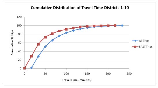
Figure 21. Distribution of Travel Times (Dist 1 – 10)
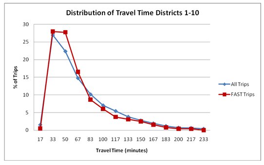
For completeness, the study team conducted similar analyses on the travel time data for trips from district 1 through district 6. The results of these analyses are presented in Figures 22 and 23. As can be seen in these graphs, the data profiles for the cumulative and individual trip travel times follow a similar pattern, suggesting that trimming of higher travel times should also be possible for the trip from the beginning of the measurement zone to the exit of US primary.
Figure 22. Cumulative Distribution of Travel Times (Dist 1 – 6)
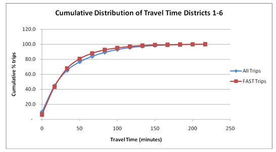
Figure 23. Distribution of Travel Times (Dist 1 – 6)
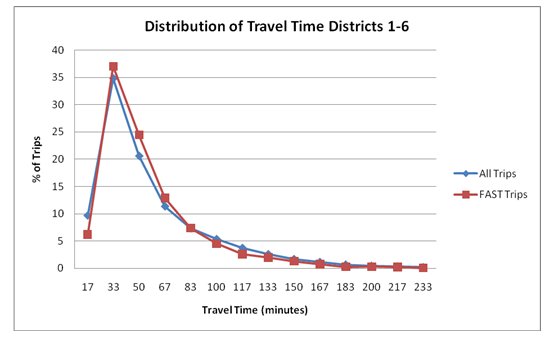
3.7 Motor Carrier Feedback
At the conclusion of the data collection period, the study team contacted the two carriers that participated in the project to gain some perspective on their operations, and to gather information related to their typical crossing experience. The principal objective was to ascertain whether the data accurately reflected the conditions they encounter when crossing into the US.
The study team first asked questions regarding the mix of loaded to unloaded trips and FAST to non-FAST trips for each carrier. The intent was to assess the ability of the GPS devices to discern the various trip types. As stated previously, trucks conducting FAST trips follow a path around the southern perimeter of the MX export compound before reaching the point where they actually cross the border and queue for entry into the US.
According to operations staff at the two carriers, the majority of US-bound trips are FAST trips. One carrier indicated that more than 90 percent of traffic was FAST trips, while the second carrier said approximately 75 percent of its US-bound trips were FAST trips. This is in contrast to the GPS data that indicated that approximately 13 percent of trips were FAST trips. While neither carrier offered detailed records to indicate that these figures were close to actual numbers, the implication is clear that the use of GPS data to isolate FAST trips is not an accurate method, at least as it was applied during the project. Further, because both carriers indicated that trucks completing FAST trips typically do not encounter queuing between MX export primary and the physical border, it is logical to conclude that the travel time within the MX export compound (district 4) is too brief to allow a large portion of the trucks to report.
The second major question the team asked the carriers was whether their drivers encounter a high degree of travel time variability when crossing into the US. As indicated previously, the recorded travel times showed a very high degree of variability, whether observing the data by time of day, day of week, or month of the year.
Representatives from both carriers concurred that there is, in fact, significant variability, and that the degree seen in the data could be accurate.27 This feedback was, of course, anecdotal in nature. As such, it does not alone validate the travel time data. It does, however, lend credibility to them. The study team asked the carriers if they had an insight into why the level of variability might be so large. They both indicated that there are several factors that can contribute to it. They suggested that travel time on days just before and just after holidays is typically unpredictable. They also stated that other factors such as significant law enforcement events-major drug interdictions, for example-can have a profound effect on screening practices, at least for a period of time.
Carriers also cited manufacturing-related events as contributors to travel time variability. Because the participating carriers do a significant amount of hauling for maquiladoras, production schedules and factory cutoffs can create spikes in volume. Finally, the carriers stated that systems problems-most notably those associated with managing the flow of documentation for US import-can slow things down. These may be systems operated by customs brokers and banks.
Both carriers cited all of the above conditions as contributing factors that complicate predicting the amount of time needed to cross.
Finally, the study team asked the carriers about the value they perceive GPS-based GPS systems have with respect to their operations. Both carriers indicated that they routinely use the tracking and tracing functions as a means to meet business needs of customers, and to satisfy shipment visibility requirements associated with compliance with C-TPAT. Both use the data on a continual basis.
4 Otay Mesa Chamber of Commerce, http://www.otaymesa.org/ab_otay/port_of_entry.html. [ Return to note 4. ]
5 Based upon data obtained from CBP at the Otay Mesa Port of Entry. [ Return to note 5. ]
6 The FAST (Free and Secure Trade) program was established by the US CBP to facilitate expedited screening at US border POEs. It requires an entire supply chain to apply for and obtain certification under the Customs-Trade Partnership Against Terrorism (C-TPAT), a program that seeks to ensure that every portion of a supply chain complies with certain minimum security assurance criteria. [ Return to note 6. ]
7 FHWA Public Roads. May 2005. http://www.ibrc.fhwa.dot.gov/publications/publicroads/05may/10.cfm. [ Return to note 7. ]
8 http://www.intelligentimagingsystems.com/ [ Return to note 8. ]
9 It is important to note that USDOT numbers are not unique to individual trucks, but are typically used as a secondary source of verification in the absence of an unobscured license plate number. [ Return to note 9. ]
10 SAFETEA-LU Section 1201, as summarized in Federal Register Vol. 72, No. 198, Monday, October 15, 2007. [ Return to note 10. ]
11 "Inrix to Deliver Real-Time Traffic Information for I-95 Corridor." GPS Daily. http://www.gpsdaily.com/reports/INRIX_To_Deliver_Real_Time_Traffic_Information_For_I_95_Corridor_999.html [ Return to note 11. ]
12 Delcan for the Baltimore Multimodal Traveler Information System Business Model. [ Return to note 12. ]
13 Delcan for the Baltimore Multimodal Traveler Information System Business Model. [ Return to note 13. ]
14 Addressing Issues with GPS Data Accuracy and Position Update Rate for Field Traffic Studies, Institute of Transportation Engineers, ITE Journal. Feb 2003; Travel Time Studies with Global Positioning and Geographic Information Systems: An Integrated Methodology, Texas Transportation Institute. 1998. [ Return to note 14. ]
15 https://ops.fhwa.dot.gov/freight/freight_analysis/perform_meas/fpmtraveltime/index.htm#travel [ Return to note 15. ]
16 Delcan for the Baltimore Multimodal Traveler Information System Business Model. [ Return to note 16. ]
17 Ferman, Martin A., Dennis E. Blumenfeld, Xiaowen Dai, "An Analytical Evaluation of a Real-Time Traffic Information System using Probe Vehicles," Journal of Intelligent Transportation Systems, 9:1, 23-34. Available at: http://dx.doi.org/10.1080/15472450590912547. [ Return to note 17. ]
18 CBP had not released statistics for March 2010 as of the writing of this report, so the 5 percent value could not be determined for that period. [ Return to note 18. ]
19 A Geofence is a virtual perimeter on a geographic area using a location-based service, so that when a telemetry device enters or exits the area a notification is generated. (Source: Wikipedia – http://en.wikipedia.org/wiki/Geofence). [ Return to note 19. ]
20 Extensible Markup Language (XML) is a simple, very flexible text format derived from SGML (ISO 8879). Originally designed to meet the challenges of large-scale electronic publishing, XML is also playing an increasingly important role in the exchange of a wide variety of data on the Web and elsewhere. (Source: W3C – http://www.w3.org/XML/) [ Return to note 20. ]
21 The set of communications protocols used for the Internet and other similar networks. It is named from two of the most important protocols in it: the Transmission Control Protocol (TCP) and the Internet Protocol (IP), which were the first two networking protocols defined in this standard. (Source: Wikipedia – http://en.wikipedia.org/wiki/Internet_Protocol_Suite) [ Return to note 21. ]
22 csv – Comma Separated Values – a file type often used to transfer data among various applications where individual values are separated by commas. [ Return to note 22. ]
23 Calmar uses its own proprietary geo-location tuning logic to improve upon the precision found in standard commercial mapping products, which Calmar considers insufficient for accurate travel time measurement. This was the case with the telemetry data acquired during the project. [ Return to note 23. ]
24 "Breadcrumb" is a term that is often used to identify points that are recorded at regular intervals by a telemetry unit as a vehicle is moving. [ Return to note 24. ]
25 GIS – Geographic Information System. A GIS is a system that allows for spatial placement and analysis of telemetry points. For this project, Calmar utilized Manifold, while Delcan used TransCAD. [ Return to note 25. ]
26 For this project, Calmar used SAS, while Delcan used a SQL database and a set of analytical algorithms. [ Return to note 26. ]
27 The carrier representatives were not shown specific numbers regarding variability. They were told, however, that the travel time might deviate by as much as 100 percent or more from the mean on a regular basis. [ Return to note 27. ]