Comprehensive Truck Size and Weight Limits Study - Highway Safety and Truck Crash Comparative Analysis Technical Report
Appendix C: Maneuvers for the Vehicle Stability and Control Analysis
This appendix documents the five maneuvers that were simulated in TruckSim® to evaluate the performance of the control and study vehicles. Each maneuver is described by a path and a speed. The avoidance maneuver required a family of similar paths. Each run of TruckSim® produced an output data file. These files were analyzed with Matlab® to calculate the desired performance parameters. Table 24 of the main report lists the performance metrics that were extracted from each of the five maneuvers and the peril that each is intended to assess.
Maneuver 1. Low-Speed Off-tracking
When a long vehicle makes a sharp turn at an urban intersection or at a right-angle intersection of two highways, the rear axles follow a path well to the inside of the steer axle path. Any instance of a trailing axle not exactly following the steer axle path is called off-tracking, and low-speed off-tracking can affect, for example, the placement of stop signs on reasonable access routes or the design of curbs on freeway entrance and exit ramps.
Path Description
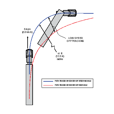
The path to assess low-speed off-tracking, illustrated in Figure C1, was the same as was used in prior work (USDOT 2000). The maneuver began with a straight path for 60 ft., long enough to establish stable motion. A curve to the right with a radius of 41 ft. began suddenly without an entry spiral. The path continued in the curve for 64.4 ft., which was a bend of 90 degrees. The path returned to a tangent, again without a spiral. The path continued for 105 ft., long enough for all vehicles to resume straight stable motion. The pavement was flat and dry with a coefficient of friction of 0.9.
Speed
This maneuver was conducted at a constant speed of 5 mph.
Analysis
The data extracted from the output file was the paths of the centerlines of each axle. TruckSim® reports the data as X-Y pairs of locations at each time step. These Cartesian coordinates were converted to polar coordinates where the origin was the center of the curve.
The analysis began at the moment the steer axle entered the curve, and it ended when the final axle passed the end of the curve.
Figure C-1. The Low-speed Off-tracking Maneuver.
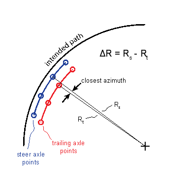
The analysis followed the path of the steer axle, which was the baseline from which deviations were measured. The analysis is illustrated in Figure C2. In outline form, the analysis steps were:
- For each point on the steer axle path, find the off-tracking of all the trailing axles.
- For each trailing axle, find the point whose azimuth is closest to the azimuth of the steer axle position. Compute the difference in radii of the trailing axle and the steer axle.
- The result is an array with one column for each trailing axle and one row for each azimuth considered. The highest value in the array is the worst off-tracking of the truck in this scenario.
If the steer axle perfectly followed the desired path, then the off-tracking of the subsequent axles would be the same as their displacement from the path. The steering model was not perfect, so the off-tracking values of drive and trailer axles were not identical to their absolute displacement values. The off-tracking was reported for the low- and high-speed off-tracking maneuvers and the transient maneuver because they are intended to measure off-tracking. The absolute displacement was reported for the two braking maneuvers because FMVSS No. 121 imposes a lane position requirement.
Figure C2. The Low-speed Off-tracking Calculation Points.
Maneuver 2. High-Speed Off-tracking
When a vehicle is on a curve on a highway, its trailing axles may follow a path identical to that of the steer axle. Or, depending on the speed, the placement of the load, the tire properties, and other factors, the trailing axles may track inside or outside of the steer axle.
The maneuver to assess the high-speed off-tracking characteristics of the vehicles was also drawn from prior work (USDOT 2000).
Path Description
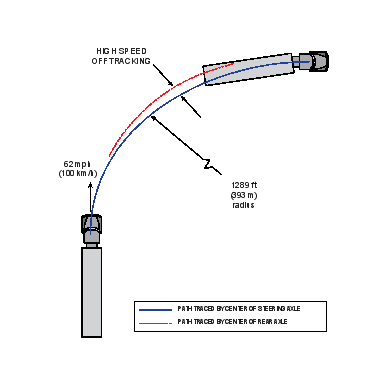
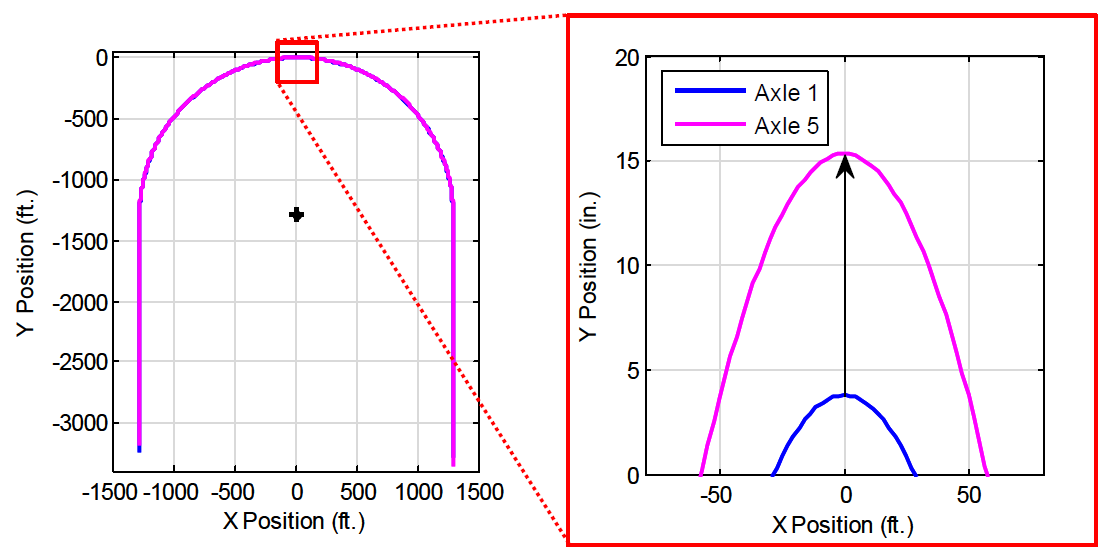
The path began with a straight segment for 2000 ft., long enough to establish stable motion. A curve to the right with a radius of 1,289 ft., as illustrated in Figure C3, began suddenly without an entry spiral. The path continued in the curve for 4,049.5 ft., which was a bend of 180 degrees. The pavement was flat and dry with a coefficient of friction of 0.9.
Figure C3. The Simulated High-speed Off-tracking Maneuver.
Speed
This maneuver was conducted at a constant speed of 62 mph.
Analysis
The data extracted from the output file were the paths of the centerlines of each axle. The data were Cartesian X-Y pairs of locations at each time step. The desired output was the steady-state off-tracking value. Steady state was reached after a few truck lengths. As each axle passed the 90-degree azimuth where the X coordinate was zero, its Y coordinate was noted as illustrated in Figure C4. The position of the steer axle was the reference. The differences of successive axle centers from the steer axle position were calculated. For all vehicle configurations, the rearmost axle demonstrated the worst off-tracking. This off-tracking value was reported in Table 26 of the main text.
Figure C4. High-speed Off-tracking Path Differences.
Maneuver 3. Straight-Line Braking
FMVSS No. 121 provides a straight-line braking test in S5.3.1.1. The conditions of the test were simulated for this maneuver, but with two exceptions. First, the straight-line braking test in S5.3.1.1 applies to a tractor with an unbraked control trailer, but the simulated vehicles were loaded according to Figure 4 of the main text, as they were for all maneuvers. In the first case for this maneuver, all axles were braked. The second exception is that two more cases were run with simulated malfunctions intended to destabilize the vehicle. One was a partial brake failure, where no braking torque was produced on the affected axle ends, and the other was an Antilock Braking System (ABS) malfunction, where tires on the affected axle ends could lock. Both failures were applied on an axle group on one side of the vehicle, to create a yaw moment. The failures were on the right side of both drive axles on the single-trailer combinations. They were on one end of the lead dolly in the multi-trailer combinations.
Path Description
This scenario used a straight path. Quoting from FMVSS No. 121, "S5.3.1.1 Stop the vehicle from 60 mph on a surface with a peak friction coefficient of 0.9 . . ."
Speed
The vehicle began at 60 mph. After the vehicle established stable motion, the service brakes were applied at 120 psi.
Analysis
These runs were analyzed two ways.
Stopping Distance
S5.3.1 of FMVSS No. 121 specifies that the beginning of the stopping distance is the "point at which movement of the service brake control begins." This was known from the TruckSim® brake control output variable, which yielded a Boolean value of 1 when brakes were applied and a Boolean value of 0 when brakes were not applied. The end of the stopping distance was the point where the speed reached 0, which was determined from the output.
Maximum Path Deviation
The lateral distance from the lane center to the center point of each axle was measured, and the peak absolute value was extracted for each vehicle simulation.
Maneuver 4. Brake in a Curve
This scenario challenged the stability of the vehicles in hard braking on a curved, wet roadway. It was based on S5.3.6 of FMVSS No. 121, which is a stopping test on a curved roadway with a peak friction coefficient of 0.5. The effect of this provision of the air brake standard is to require ABS. As with the straight-line braking scenario, this scenario was run with normally functioning brakes on all axle ends and with brake failures and ABS malfunctions in the positions most likely to produce instability.
Path Description
The maneuver was conducted on a continuous curve with a radius of 500 ft.
Speed
The vehicle began at 30 mph. After the vehicle established stable motion, a full-treadle (120 psi) brake application began.
Analysis
These runs were analyzed three ways.
Stopping distance
Although it is not a requirement of this test in FMVSS No. 121, the stopping distance for every vehicle was measured as it was in the straight-line braking test.
Maximum Path Deviation
This was calculated and reported as in the straight-line braking test. The Cartesian coordinates were converted to polar coordinates where the origin was the center of the curve. The path deviation of each axle was calculated as the radius of the axle center minus the radius of the lane center.
Lateral Load Transfer Ratio
This was a measure of the roll stability of the vehicle. It was the amount of vertical load that was transferred from the tires on the axle end on the inside of the curve to those on the outside. Mathematically, the formula for calculating the Lateral Load Transfer Ratio of an axle is shown in Equation C1.
![]() (C1)
(C1)
where
FL is the force on the left side tires and
FR is the force on the right side tires.
When an evenly loaded vehicle is driving straight on level road, the ratio is 0. When the load on one end of the axle is completely removed, the ratio is 1. A ratio of 1 does not necessarily mean the vehicle rolled over. Whether a vehicle actually rolls over depends on its roll rate, how long the vehicle remains in the curve, and other factors.
The Lateral Load Transfer Ratio was calculated as a function of time for all axles. The peak value for each axle was extracted. The rearmost axle had the worst ratio in all cases.
The lateral load transfer has a steady-state value while the vehicle is at a steady speed in the curve, and the quantity begins to decrease when the brakes are applied. In nearly every case, the quantity reported was the steady-state value. The figures in Appendix F show a transient about 1 second after the brakes were applied. In only one case did the transient exceed the steady pre-braking value, but then only minimally.
Maneuver 5. Avoidance Maneuver
The procedure to evaluate rearward amplification properties was based on the single lane change maneuver in ISO 14791 (ISO 2000).
Path Description
The path began with a straight segment for 350 ft., long enough to establish stable motion. The maneuvering section of the path is a single lane change. Section 7.5.2 of the standard calls for the steering input to be followed by 5 seconds of neutral steering.
The standard allows either an open-loop hand wheel input (7.5.2) or closed-loop path (7.5.3) to effect the lane change. Maneuvers were run with closed-loop path-following control. The TruckSim® driver model's preview time was set to 0.15 seconds, which was found to yield the best results. The expression for the closed-loop path is
![]() (C2)
(C2)
where
y is the lateral position
a is the desired peak lateral acceleration
ω is the frequency of excitation
x is the distance traveled down range ("station")
v is the forward speed of the vehicle.
The quantity ω•x/v ranges from 0 to 2Π to provide one cycle of lateral acceleration input. Figure C5 shows a typical path of a simulated tractor and the corresponding lateral acceleration.
Figure C5. Control Double Vehicle Path While Executing the 12-ft. Lane Change Maneuver
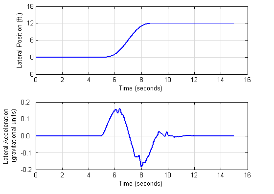
Section 7.3 recommends a peak lateral acceleration of 2 meters/second2 (approximately 0.2 gravitational units) but permits a lower maximum when appropriate. A peak of 0.15 gravitational units was selected for this study.
The peak lateral acceleration and frequency of the maneuver vary slightly from the ideal quantities in Equation C2 because the TruckSim® driver model does not perfectly follow the intended path (although the greatest imperfection in any of the runs was 1.6 in.). The resulting spread of frequencies was sufficient to identify a peak response in the measured quantity in nearly every case. The actual peak acceleration amplitude ranged from 0.13 to 0.19 gravitational units, so the tests were satisfactory.
This is the only scenario that needed iteration: Section 7.5.1 of the standard calls for the test to be conducted for at least three frequencies to find the maximum rearward amplification. Runs were conducted at eight frequencies. With the peak acceleration fixed, then the frequency and lateral offset are inversely related:
![]() (C3)
(C3)
Eight paths were developed following Equation C2. The offset of the lane change (y at the end of the maneuver) ranged from 3 ft. to 24 ft. as listed in Table C1. The desired peak lateral acceleration (a) was 0.15 gravitational units and the forward speed (v) was 50 mph in all cases. The resulting frequency of excitation (ω/(2Π)) of each path and the longitudinal distance required to complete the path (Δx) are also listed in the table.
Speed
This maneuver was conducted at a constant speed of 50 mph.
Analysis
These runs were analyzed for three quantities-off-tracking, rearward amplification of lateral acceleration and lateral load transfer ratio. Every vehicle was run through the eight lane changes in Table C1. The three analysis quantities were calculated at each of the eight lane change distances, corresponding to eight excitation frequencies as in the table. The highest of these eight values was reported as the result in Table 29 of the main text. Graphs of all quantities are in Appendix E.
Off-tracking
Section 8.3 of the standard defines off-tracking for the maneuver. The analysis followed the path of the steer axle, which was the baseline from which deviations were measured. The analysis is illustrated in Figure C6. In text form, the analysis was as follows:
- For each point on the steer axle path, find the off-tracking of all the trailing axles.
- For each trailing axle, find the point whose X value (station) is closest to the X value of the steer axle position. Compute the difference in Y values (lane position) of the trailing axle and the steer axle.
- The result is an array with one column for each trailing axle and one row for each station position considered. The highest value in the array is the worst off-tracking of the truck in this scenario.
Figure C6 plots the path of each axle center for a 12-ft. lane change for the control double vehicle. Off-tracking was computed as the difference in Y values (lane position) of each trailing axle from the steer axle. The worst off-tracking of the truck at this excitation frequency was 12.75 - 11.42 or 1.33 ft., which was reported as 16 in. This process was repeated for the eight excitation frequencies in order to find the global highest absolute off-tracking value.
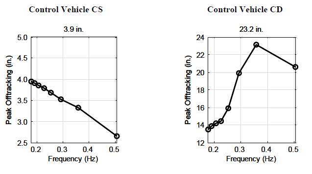
Figure C7 plots peak off-tracking for the control single and control double vehicles for all eight excitation frequencies listed in Table C1. The graph shows that the control double vehicle demonstrated peak off-tracking of 23.2 in. at an excitation frequency of 0.36 Hz, which was the 6-ft. lane change.
Figure C6. Control Double Vehicle Off-tracking Calculation for the 12-ft. Lane Change
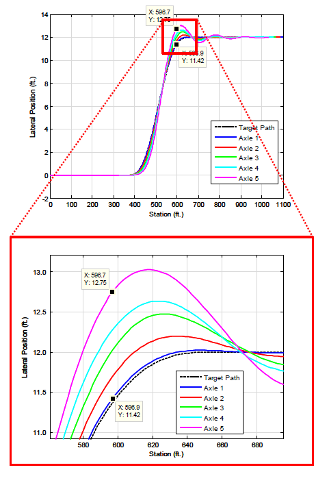
Figure C-7. Maximum Off-tracking for All Excitation Frequencies
Rearward Amplification
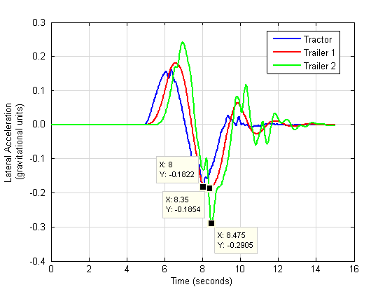
Figure C8 shows the lateral acceleration time histories of the tractor and two trailers of the control double vehicle in the 12-ft. lane change. Markers in the figure identify the maximum of each unit's acceleration. The rearward amplification is the ratio of the peak lateral acceleration of the rear trailer to that of the tractor.
A low-pass digital Butterworth filter (fourth order filter, 5-Hz cutoff frequency) was applied to the TruckSim® lateral acceleration output data to attenuate high-frequency spikes in the data.
Figure C8. Rearward Amplification Reflected by Peak Lateral Acceleration in Trailers
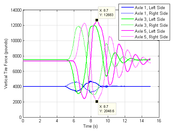
Lateral Load Transfer Ratio
Load transfer ratio was calculated in the same manner as it was for the brake-in-a-curve maneuver, using Equation C1.
Figure C9 plots the vertical forces on the tires for a 12-ft. lane change for the control double vehicle. (These are forces on the axle end. The steer tires have the forces plotted; other axles have dual tires so the force on each tire is half of the value.) The peak Lateral Load Transfer Ratio occurred at a peak in the path, as shown in this figure.
C9. Shifts in Vertical Tire Force Over Time Reflect Vehicle "Leaning" during the Modeled Avoidance Maneuver.