Appendix 2. Economic Framework
Appendix 2 provides an overview of the microeconomic framework developed in previous study within which the freight-related economic benefits and costs of transportation improvements can be measured. A key objective of the framework is to ensure that BCAs recognize the gains in economic welfare that follow from the propensity of industry to adopt productivity-enhancing "advanced logistics" in response to transportation infrastructure improvements.
Framing the Problem
The term logistics pertains to the way firms organize themselves in relation to transportation, warehousing, inventories, customer service and information processing. The phrase "advanced logistics" is shorthand for technologies and business processes that permit firms to reduce costs by substituting transportation, e-commerce, and just-in-time deliveries for large inventories, multiple warehouses, and customer service outlets. Firms can reorganize in response to transportation infrastructure improvements to reap the rewards of advanced logistics.
Investment in highway improvement projects, both infrastructure and info-structure, will affect attributes of links within the U.S. freight transportation system. For example, flow capacity may be increased by the addition of more lanes, increases in speed limits, limited access highways, and operational/ITS improvements. There also may be fewer restrictions on truck weights and improved bridge clearances. Further improvements could be made to ports/customs processes that lead to increases in net system traffic flow. These types of improvements result in travel-time savings and increased reliability. These and other downstream effects are shown diagrammatically in Figure 7. Productivity gains occur within industries at the level of the firm. The potential for firms to reorganize their logistics systems and policies will occur according to specific trade-offs between logistics components.
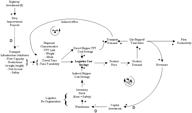
Figure 7. Freight Economics Influence Diagram
Nature of Reorganization
Logistics systems are key enablers of economic development. Governments can adopt policies that will encourage overall logistics efficiency. In some instances, logistics costs can amount to 30% of delivered costs. In efficient economies, these costs can be as low as 9.5%.[7] Transportation charges account for nearly 40% of all logistics costs. Trucks also serve as the access and egress mode for maritime, air, intermodal, and many rail trips. Short haul trips are therefore an essential component of the economy.
Logistics costs are driven by activities that support the logistics process. Trade-offs are possible among the elements of logistics costs in order to minimize total costs given customer service level objectives. The main components of logistics costs are:
- Transportation costs
- Warehousing costs
- Order processing/information systems costs
- Lot quantity costs
- Inventory carrying costs
These elements are inter-related, and various trade-offs exist. It is worth noting that some of these trade-offs are not realized in a continuous way. Consolidation of warehouses occurs at a discrete point in time and will be different for various firms based on their decision to invest in new logistics systems. The primary goal of a firm in developing its logistics strategy is to provide customer service while reducing costs, thereby increasing profits and competitiveness.
Changes in Logistics Network Infrastructure
A firm could re-organize its logistics in many ways as a result of lower transportation costs. For example, it could reduce the number of warehouses and increase the use of transportation services. Four factors influence the number of warehouses a firm chooses to maintain: 1) cost of lost sales, 2) inventory costs, 3) warehousing costs, and 4) transportation costs.
- Cost of Lost Sales. The cost of lost sales is the most difficult to quantify. It generally decreases with the number of warehouses and varies by industry, company, product, and customer. The remaining cost components are more consistent across firms and industries.
- Inventory Costs. Inventory costs increase with the number of warehouses because firms maintain a safety stock of most or all products at each facility.
- Warehousing Costs. More warehouses mean more space owned, leased, or rented. Fixed costs across many facilities are larger than the marginal variable costs of fewer locations.
- Transportation Costs. Transportation costs initially decline as the number of facilities increases due to proximity. Costs eventually increase when a firm maintains too many warehouses due to the combination of inbound and outbound transport costs.
A firm seeking to minimize total costs, which is the sum of the above components, could balance all cost components by solving a multi-facility location problem (as depicted in Figure 8). As transportation costs decline, possibly due to highway infrastructure investment, the minimum total cost generally will be achieved by maintaining fewer warehouses. The nature and timing of reorganization will occur at different points for each firm. Sufficient potential gains will need to be realized before an investment hurdle rate is exceeded.
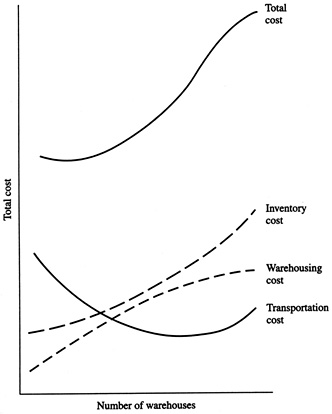
Figure 8. Relationship between Total Logistics Cost and Number of Warehouses Due to Changes in Inventory Policy
A simpler, more rapid response to lower transportation costs, improved transit times, and reduced delivery time variability is a change in a firm's inventory policy. To demonstrate the direct relevance of travel time and travel-time variability on total logistics costs, consider a simple example where a firm has a central production plant and a single warehouse located within its market area such as in Figure 9.
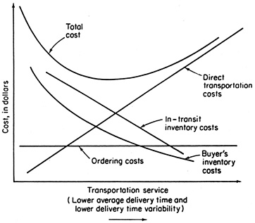
Figure 9. Generalized Cost Trade-offs for Transportation Services
As direct transportations costs decrease, the minimum total logistics cost point moves to the right. A profit-maximizing firm would increase the demand for transportation services. An increase in travel time and variability can be costly. Money tied up in inventory isn't earning interest. The longer it takes to ship perishable goods, the more they depreciate. It's the near elimination of travel-time variability that makes just-in-time inventory management possible. Figure 10 presents the basic inventory cost trade-offs.
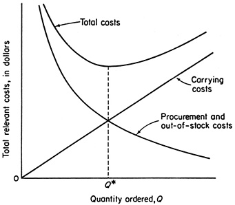
Figure 10. Basic Inventory Cost Trade-offs
Stockout and backorder costs[8] are a function of the lead-time distribution of supply. Lead times are a function of travel-time and travel-time variability (i.e., reliability) as shown in Figure 11. Reductions in either travel-time and/or travel-time variability will directly impact various logistics cost components and may trigger reorganization at the level of the firm. Shorter and more predictable lead times can enable firms to reduce their reorder points and average stock levels while maintaining the same level of service. This reduces logistics carrying costs.
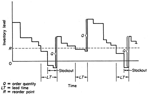
Figure 11. Inventory Levels Under a Fixed Order Quantity-Variable Order Interval Policy
A paper by Mohring and Williamson[9] provides a formal analysis of "reorganization effects," the adjustments in logistical arrangements that shippers make in response to lower costs of freight movement. Typically, these adjustments involve fewer warehouses and more miles of truck movement as shippers take advantage of lower freight costs to consolidate storage facilities and reduce inventory costs. These effects are the principal source of benefits not captured in the conventional approach to BCA.
The ability of a firm to exploit manufacturing scale economies can be limited by the cost of transporting its products to market. A reduction in unit transportation costs can yield two types of benefits. First, it provides "direct" benefits by reducing the costs of distributing the outputs of existing manufacturing facilities. Second, a transport-cost reduction can make it more efficient to expand the outputs and marketing areas of individual production facilities and take greater advantage of manufacturing scale economies. This use of more transportation intensive means of production and distribution in response to reduced transportation costs generates "reorganization" benefits.
Logistics management continues to evolve with the adoption of e-business practices and various forms of JIT delivery. E-commerce and e-business will increase trade. Growing trade means more freight movements. Note that the nature of these movements may evolve to more single-package deliveries requiring additional transport services. New information technologies also enable JIT logistics systems that rely on dependable and inexpensive transportation. E-business may affect the nature and extent of transportation demand as well as the rate of industrial reorganization, but the logistics principles remain the same.
Microeconomic Framework
The framework developed is general in the sense that it captures benefits of any highway improvement.[10] The introduction of ITS, for instance, to manage congestion would translate into reduced travel times and enhancing reliability. Benefits of any initiative affecting overall logistics costs, such as vehicle operating limits, could be considered within the context of the framework that is presented in this sub-section.
Approach
In Measuring the Relationship between Freight Transportation and industry Productivity,[11] a method was developed to estimate the elasticity of logistics cost with respect to travel-time savings, call it  . This quantity was derived from a sample of firms' responses (cost savings) to travel-time improvements. A similar approach can be used to determine a firm's elasticity of demand for transportation as a result of travel-time savings and changes in logistics, call it
 ![]() . This last quantity encapsulates the firm's response to highway improvements in terms of new transportation demand as a result of possible substitutions. The quantity is shown in Figure 12 for a sample of several firms. The points at which reorganization occurs,
. This last quantity encapsulates the firm's response to highway improvements in terms of new transportation demand as a result of possible substitutions. The quantity is shown in Figure 12 for a sample of several firms. The points at which reorganization occurs,![]() Wi, may be specific to individual firms. The trend will allow the inference of effects (slope of the curve) over a range of firms.
Wi, may be specific to individual firms. The trend will allow the inference of effects (slope of the curve) over a range of firms.
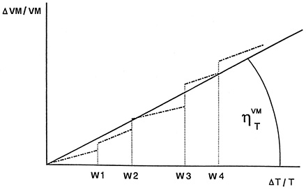
Figure 12. Aggregate Relative Change in Transportation Demand
To calculate benefits of road improvements, the elasticity of transportation demand with respect to transportation cost ![]() is required. A simple relationship can be established between these two elements as follows:
is required. A simple relationship can be established between these two elements as follows:
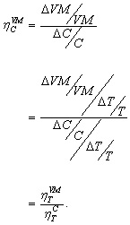
This expression is the ratio of the elasticity of transport demand with respect to travel time ![]() , and the elasticity of transportation cost with respect to travel time . Both of these might be estimated using a suitable sampling methodology within various industries.
, and the elasticity of transportation cost with respect to travel time . Both of these might be estimated using a suitable sampling methodology within various industries.
Estimation of transportation user costs should not present a problem. For instance, assuming that wages accounted for 30% of transport operating costs, a 20% decrease in travel time could result in a 6% decrease of direct transportation cost per vehicle mile. In reality, other substitutions could also take place.
The fundamental determination of the demand curve for transportation services involves two quantities, price and vehicle miles used/traveled. The change in each of these components was derived as a function of some third dimension, travel time and/or travel time variability. This third dimension is a function of highway investment. Once time savings are known or estimated, logistics cost savings estimation can be carried out at the firm level to include logistics reorganization effects. Each firm is different, but with a representative sample, the general response trend can be quantified over specific industries. Note that the third dimension could also include changes in vehicle capacity or service hours, thereby increasing freight throughput. This approach has the added advantage that the demand for transportation services can be aggregated across markets or commodities and therefore facilitating benefits estimation for highway-network improvements. Aggregation using a product demand curve may be difficult due to the varying nature of products.
Changes in Output/Product
Demand The demand for freight services is derived from the demand for final products carried. Because freight transport is closely related to land-use patterns, it is also important to consider influences affecting industrial location and distribution. Transport demand could thus increase due to two effects. First, logistics reorganization may result in substitution of additional transport for inventory and holding locations. Second, savings from lower transportation and overall logistics costs may be passed on to consumers and result in an increase of consumer product demand. This increase in demand is embodied in increases in transportation services required. Both these components must be part of the effective demand upon which net benefits are derived.
Competitive Market
The benefits of infrastructure investment can be derived from the change in consumer surplus for transportation demand. In general form, it is possible to write:
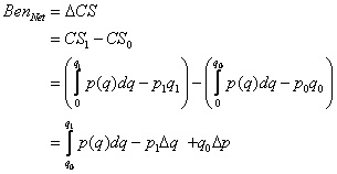
In this case, price![]() p(q) = C(VM) is the cost of transport per vehicle mile at a level of demand
p(q) = C(VM) is the cost of transport per vehicle mile at a level of demand![]() q = VM. This general expression encapsulates the net benefit of the infrastructure improvement in the absence of marginal cost pricing.
q = VM. This general expression encapsulates the net benefit of the infrastructure improvement in the absence of marginal cost pricing.
One approach to evaluating the integral above would be to assume constant elasticity of demand near the present demand level. A general expression for a constant-elasticity-of-demand schedule is![]() Q = a/Pb where Q is the quantity sold at a price of P and where a and b are constants.
Q = a/Pb where Q is the quantity sold at a price of P and where a and b are constants.
Monopoly
In the case of a monopoly, it was shown that net benefits involve both a consumer's gain as well as a producer's gain. This is true for transportation and other markets.
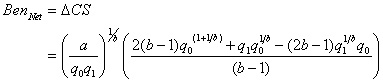
BenNet = ΔCS + ΔCS′
The consumer's gain is![]() ΔCS. The producer's gain
ΔCS. The producer's gain![]() ΔCS′ has the exact same form, except that the price is replaced by marginal revenue
ΔCS′ has the exact same form, except that the price is replaced by marginal revenue ![]() . The new price, which maximizes the monopolist's profit, can be approximated as
. The new price, which maximizes the monopolist's profit, can be approximated as![]() B = A – ΔCLog. These two areas are illustrated graphically below. In the case of a monopoly, two areas must be considered, but the overall procedure for each is the same. The expression is:
B = A – ΔCLog. These two areas are illustrated graphically below. In the case of a monopoly, two areas must be considered, but the overall procedure for each is the same. The expression is:
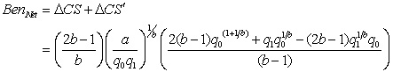
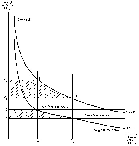
Figure 13. Benefits in the Presence of Monopoly
Accounting for Non-Marginal Cost Pricing
A simple adaptation of the cost-benefit methodology can be used to correct for non-marginal cost pricing. If TC is the total cost of providing a road with N trips made along it per unit time, then this total cost can be defined as:
where C is the cost of one trip to a vehicle and![]() ƒ(K) is the cost per time period of providing K units of road capacity. The short term marginal cost becomes:
ƒ(K) is the cost per time period of providing K units of road capacity. The short term marginal cost becomes:
The![]() Nth vehicle then incurs a cost itself and imposes a cost on other users. This is demonstrated graphically in Figure 14.
Nth vehicle then incurs a cost itself and imposes a cost on other users. This is demonstrated graphically in Figure 14.
The CBA could be revised with estimated marginal social cost prices for the use of transport services at a given level of use. These estimated price adjustments could have a wide margin of uncertainty. However, if a highway improvement option remains justified and highly ranked compared to other competing alternatives in the presence of approximate marginal cost pricing, then there is good confidence that the option valuations are robust to underlying assumptions. The actual estimation of marginal cost prices is work to be carried out as part of a follow-on task.
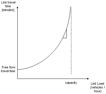
Figure 14. Typical User Link Travel Time Graph and Marginal Cost
Approach Summary
In summary, the microeconomic framework rests on estimating the change in consumer surplus reflected in the 'shift' in the demand curve for freight transport that follows the improvement. This provides significant added value to previous research such as the 'shift' in the demand curve now reflects increasing output as well as trade-offs between transportation spending and total logistics costs.
- Roberts, P.O. Logistics Supply Chain Management: New Directions for Developing Economies, on behalf of the World Bank, Feb. 1999.
- Stockout periods occur when a product is not available. A key element of customer service, stockout periods can lead to out-of-stock costs incurred when an order is placed but cannot be filled from inventory. These costs can be classified as lost-sales costs and back-order costs. Back-orders often generate additional order processing as well as transportation costs when they are not filled through the normal distribution channel.
- Mohring, H., Williamson, H.F. "Scale and Industrial reorganization economies of transport improvements," Journal of Transport Economics and Policy, Sept. 1969.
- Both infrastructure and info-structure changes.
- NCHRP 2-17(4), Measuring the Relationship between Freight Transportation and industry Productivity, Final Report, HLB Decision Economics Inc., June 1995.