Comprehensive Truck Size and Weight Limits Study - Data Acquisition and Technical Analysis Plan
1.1 Task Objective
The Data Acquisition and Technical Analysis Plan (Task III: Data Acquisition and Technical Analysis Plan, U.S. Department of Transportation (USDOT) Comprehensive Truck Size and Weight (2014 CTSW) Limits Study) provides an outline as to the types of data and models that were acquired and analyzed. This plan includes the 2014 CTSW Study’s:
- Scenario description
- High level workflow by task
- Data/model accessibility and data custody guidelines
- Generic Data agreement
- Types of data that will be analyzed, per task
- Sources for each data type, including software used to generate data for analysis
- Additional limits or restrictions for sharing task data, beyond the assumptions stated in the data use agreement
Truck Size and Weight Scenarios
Potential modal shifts associated with the six different truck configurations and highway networks their operation was assessed on (scenarios) were analyzed in this 2014 CTSW Study. Each involved estimating the impacts of changes in federal law that would allow specific vehicle configurations to operate at gross vehicle weight (GVW) limits above the current 80,000 pound federal weight limit or beyond current federal length limits. Table 1 shows the vehicles assessed under each scenario as well as the current vehicle configuration used to conduct the assessments with (the control vehicle).
April 2016 Report to Congress, Comprehensive Truck Size and Weight Limits Study, Moving Ahead for Progress in the 21st Century (MAP-21) Act.
Note: For improved clarity in the network description, this table replaces earlier versions.
The first three scenarios allow heavier tractor semitrailers than are generally allowed under currently federal law. Scenario 1 assesses the impacts of a 5-axle (3-S2) tractor-semitrailer to operate at a GVW of 88,000 pound while Scenarios 2 and 3 would assess the impacts of (3-S3) 6-axle tractor semitrailers operating at GVWs of 91,000 and 97,000 pounds, respectively. The control vehicle for these scenario vehicles is the 5-axle tractor-semitrailer with a maximum GVW of 80,000 pounds. This is the most common vehicle configuration used in long-haul over-the-road operations and carries the same kinds of commodities expected to be carried in the scenario vehicles.
Scenarios 4, 5, and 6 assess the impacts of commercial motor vehicles that would serve primarily less-than-truckload (LTL) traffic that currently is carried predominantly in 5-axle (3-S2) tractor-semitrailers and 5-axle (2-S1-2) twin trailer combinations with 28 or 28.5-foot trailers and a maximum GVW of 80,000 pounds. Scenario 4 examines a 5-axle (2-S1-2) double trailer combination with 33-foot trailers with a maximum GVW of 80,000 pounds. Scenarios 5 and 6 include triple trailer combinations with 28.5-foot trailer lengths and maximum GVWs of 105,500 (2-S1-2-2) and 129,000 (3-S2-2-2) pounds, respectively. The 5-axle twin trailer with 28.5-foot trailers is the control vehicle for Scenarios 4, 5, and 6 since it operates in much the same way as the scenario vehicles are expected to operate.
With the exception of the triple trailer combinations, the scenario vehicles were assumed to be able to travel wherever their control vehicles could operate. For analytical purposes triple trailer combinations are assumed to be restricted to a 74,500 mile network of Interstate and other access-controlled principal arterial highways. Access off this network to terminals and facilities for food, fuel, rest, and repairs was restricted to a maximum of 2 miles. These restrictions recognize that the length and stability and control properties of triples would not make them suitable for travel on roads with narrow lanes or restrictive geometry.
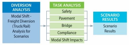
Figure 1 provides a high level workflow of the entire 2014 CTSW Study by the five technical compiled reports. In general, the modal shift freight diversion analysis for truck/truck and rail/truck by scenario served as input to the five technical compiled reports (safety, pavement, bridge, compliance, and modal shift impact including energy, emissions, traffic operations, rail contribution). The analyses completed under these Study areas provided the scenario results for the 2014 CTSW Study.
Figure 1: High Level 2014 CTSW Study Work Flowchart by Task
1.2 Data and Model Requirements for Each Task Area
The data requirements for each of the five study areas (safety, pavement, bridge, compliance, and modal shift) are contained in this section of the document. For a more complete understanding of how and why the data was used in the 2014 CTSW Study, refer to the individual Technical Reports. Table 2 summarizes the models and data used by task area.
Table 3 provides the 2014 CTSW Study’s data/model accessibility and data custody guidelines. Data and models used in the 2014 CTSW Study met the following requirement, “can it (data/models) be made accessible to a third party.” Table 3 provides that accessibility for each type of data and model that was used in the 2014 CTSW Study.
Additionally, the data custody guidelines were designed and applied during the conduct of the Study when using private/proprietary data. The use of such data needed to be transparent and accessible within the data agreement. Table 3 provides the specific private/proprietary data custody guidelines for the 2014 CTSW Study.
The generic data use agreement was used for private/proprietary data providers in the Study. Table 4 shows the generic safety data agreement.
Common Data Uses
The entire 2014 CTSW Study analysis for the five technical compiled reports (safety, pavement, bridge, compliance, and modal shift) shared a common set of data for the base case as well as for the six scenarios. The common data is vehicle miles of travel (VMT) for the base case in 2011. The base case VMT (reflecting the current fleet’s use of the highway network system) was used in the modal shift analysis area to estimate the change in VMT for each of the alternative truck configurations (six scenarios) introduced into the existing fleet.
Modal shift analysis included both shifts between the truck and rail modes and shifts in truck types and various operating weights within the truck mode.
The modal shift analysis provided the foundation for assessing the full range of potential impacts associated with the truck size and weight scenarios analyzed in this 2014 CTSW Study. Changes in allowable vehicle weights and dimensions influenced the payloads that can be carried on different truck configurations which in turn affected:
- The total number of trips and miles of travel required to haul a given quantity of freight
- The transportation mode chosen to haul different types of freight between different origins and destinations
- The truck configurations and weights used to haul different types of commodities
- The axle loadings to which pavements and bridges are subjected
- Potential highway safety risks
- The costs of enforcing federal truck size and weight limits
- Energy requirements to haul the nation’s freight
- Emissions harmful to the environment and to public health
- Traffic operations on different parts of the highway system
- Total transportation and logistics costs to move freight by surface transportation modes
- The productivity of different industries
- The competitiveness of different segments of the surface transportation industry
These various impacts are discussed in each of the five Technical Reports (safety, pavement, bridge, compliance, and modal shift impacts) in this 2014 CTSW Study. Impacts are quantified to the greatest extent possible, but where data are unavailable to reliably quantify potential nationwide impacts, qualitative assessments of the impacts of changes in truck size and weight limits are discussed.
The modal shift analysis was comprised of the following elements:
- Developed a detailed project plan describing how the modal shift analysis was conducted using analytical tools and data identified in the desk scan.
- Estimated truck traffic currently operating within and above existing federal truck size and weight regulations.
- Specified truck size and weight scenarios for analysis in the 2014 CTSW Study. The basic vehicle configurations to be analyzed in the 2014 CTSW Study were identified by USDOT, butspecifications for those vehicles and how they would operate were developed for use in the various study areas.
- Developed assumptions necessary for the modal shift analysis and identify limitations in the data and analytical methods that will affect the analysis.
- Estimated modal shifts associated with each scenario using the analytical tools and data chosen for the analysis.
- Shared the modal shift estimates with each of the five technical compiled areas (safety, pavement, bridge, compliance, and modal shift impacts) for analysis and results of the six scenarios.
A complete summary of the modal shift common data assumptions, limitations, and results can be found in the Modal Shift Comparative Analysis Technical Report. Use of the modal shift scenario estimates for analysis and results can be found in each of the five Technical Reports.
1.2.1 Task V.A. Highway Safety and Truck Crash Analysis: Data Requirements
The proposed approach to meet the requirements of the safety analysis required a variety of data for the crash analysis, vehicle stability and control analysis, and the inspection/violation analysis.
1.2.1.1 Crash Data Analysis – Method 1: Route-Based Method Data Needs
Several states (Ohio, Indiana, Maine, and Louisiana) were identified that could be possible candidates for this method. State permitting offices in many states were contacted to help identify potential routes. The enforcement agencies in the states were also contacted, which should have insights on where various configurations are traveling. Finally, WIM experts were also closely worked with to determine the level of exposure data available for the analysis, including the location of specific WIM stations on routes of interest. As part of the decision-making process, the extent of the mileage available in each state where reference trucks are traveling was taken into account. It is recognized that the mileage available in some states is limited, and that care must be taken when attempting to extrapolate the results from these locations to a more extensive network of roadways. At the same time, the selection was limited by the locations where the reference configurations are presently operating.
1.2.1.2 Crash Data Analysis – Method 2: Fleet-Based Method Data Needs
The availability of fleet data for use in the safety analysis in the 2014 CTSW Study was pursued. Working through the American Trucking Associations (ATA) and the American Transportation Research Institute (ATRI), carrier contacts were established and pursued for crash and operations data reflecting triples operations and legal divisible heavy trucks (i.e., those regularly operating over 80,000 pounds). Two types of analyses were proposed: 1) a comparison of triples safety (i.e., three 28.5 ft trailers) compared to doubles (two 28.5 ft. semitrailers) and 2) a comparison of the heavy legal vehicles compared to a 3-S2 80,000 pounds configuration.
In the 2014 CTSW Study application Method 2, the Safety Performance Functions (SPF) was developed from the crash and exposure data for baseline vehicles provided by carriers. The effect of future vehicles were estimated by comparing the crashes experienced with the future vehicles compared to the SPF developed from baseline vehicles using negative binomial regression This is the basic formulation to be pursued; the team explored other options, data permitting.
Data Request and Data Custody
The data requests for legal divisible heavy trucks and triples analysis were developed. The basic data elements requested from both groups of carriers included:
- Date of crash – would prefer historical data back to 2006 if possible.
- Time of Day
- Location of crash (street address; interstate highway; state route number and milepost or other location reference).
- State
- Number injured in truck
- Number injured in other involved vehicle
- Number killed in truck
- Number killed in other involved vehicle
- Truck driver age
- Truck driver experience with firm
- Type of collision
- Truck rear-ending passenger vehicle
- Passenger vehicle rear ending truck
- Truck crossing center median (head on)
- Passenger vehicle crossing center median (head on)
- Truck striking passenger vehicle (other)
- Passenger vehicle striking truck (other)
- Truck single-vehicle crash
- Driver-related factors in crash
- Vehicle-related factors in crash
- Roadway/weather related factors in crash
- Seat belt use
- Truck driver
- Passenger vehicle driver and passengers
- Driver and vehicle violations - truck
- Driver-related factors - passenger car
1.2.1.3 Crash Data Analysis – Method 3: State Crash Rate Analysis Data Needs
Both the fleet-based and the route-based methods are aimed at comparing the crash-based level of safety for future truck configurations with current baseline trucks. Depending on the level of detail and amount of data available for both these methods, difficulties in developing estimates of crash increases or decreases for each individual scenario truck configuration were encountered. In an attempt to develop specific safety estimates for each scenario configuration, an analysis was conducted based on crash and exposure data from individual states.
The crash data, roadway inventory data and AADT data for 2008-2012 was acquired for both the triples and heavies (tractor-semitrailers with GVWs greater than 80,000 pounds) study for each state chosen. Eight candidate states were identified – Oregon, Kansas, Nevada and Utah for the triples study, Washington, North Dakota and Maine for the heavy semitrailers study, and Idaho for both. Washington and Maine crash, inventory and AADT data was available from the Highway Safety Information System (HSIS). NHTSA’s State Data System (SDS) had captured multiple years of crash data from certain states. Some states will allow non-NHTSA access to their data with prior permission. Current SDS information indicates the following:
- Triples study
- Idaho – No SDS data. Data was obtained from Idaho.
- Oregon – No SDS data. Data was obtained from Oregon.
- Kansas – 2008 data available with permission in SDS. 2009 -2012 data was obtained from Kansas.
- Nevada – No SDS data. Data was obtained from Nevada.
- Utah – No SDS data. Data was obtained from Utah.
- Heavies study
- Michigan – 2008-2009 data available with permission in SDS. 2010-2012 data was obtained from Michigan.
- Idaho – No SDS data. Data was obtained from Idaho.
- Washington – Available in HSIS.
- Kentucky – 2008-2010 data available with permission in SDS. 2011 -2012 data was obtained from Kentucky.
- Maine – Available in HSIS.
In general, SDS was not a useful source of crash data for this study. All years of crash data for the chosen states were collected from those states.
Except for Washington and Maine, roadway inventory and AADT data was obtained directly from the chosen states. It is noted that states generally only retain current year inventory data, but usually do retain historical AADT data.
Except for Washington and Maine where customized analysis files were obtained from HSIS, the development of state analysis files required significant effort. Crashes involving the trucks to be analyzed were linked with roadway segments in order to link with AADT data. WIM station data (perhaps with a different linear reference system than the crash and inventory/AADT data) was linked to the roadway segments and extrapolated to longer study segments. Except for the WIM data, linking, merging and using state-based crash, inventory and AADT data was conducted. This effort was conducted in formulating procedures to make this complex process as efficient as possible.
1.2.1.4 Vehicle Stability and Control Analysis Data Needs
Data to support this subtask came from a number of sources. Members of the safety team have validated models of heavy vehicles in many configurations that approximate those being considered. Inputs also came from connections with industry or inquiries to appropriate personnel in FHWA. Publications were consulted as necessary.
1.2.1.5 Safety Inspection and Violation Analysis Data Needs
The use of current, accurate data and up-to-date, effective modeling tools was critical to the success of this project. The USDOT was in possession of a number of national datasets related to commercial vehicle operations. For example, data from Commercial Driver’s License Information System (CDLIS) provided information on the type of licenses that exist among commercial drivers (number of Class A, B, and C, with special restrictions/exemptions to exceed Federal weight limits). Multi-year data from the Motor Carrier Management Information Systems (MCMIS) was relevant for identifying crashes and inspection violations that may be associated with weight and size limits. The inspection file contained a field for GVW, which was particularly useful for segmenting truck configurations. This database also contained company safety profiles.
As part of this subtask, a literature review was conducted to identify factors associated with truck weight and size violations. Based on these past studies and discussions with experts in the field, a list of the variables needed to conduct the safety inspection and violations analysis and identified the national databases to obtain the data was prepared.
1.2.2 Task V.B. Pavement Analysis: Data Requirements
The proposed approach in the Pavement Comparative Analysis study area to meet the requirements of the pavement analysis task required a variety of data inputs, some of which are precisely the same data required by other tasks, and some of which are either unique to this task or required more detail than the other tasks.
1.2.2.1 Pavement Design and Materials Data: AASHTOWare Pavement ME Design® required a large number of pavement design details, soil data, and other materials data. The software package included the climate data needed for proper program operation, and included a large quantity of nationally-derived default data for nearly everything else. To properly analyze the sample pavement sections, however, materials and design parameters were carefully matched to typical in-use pavement sections in each climate zone and at each traffic level.
1.2.2.2 Vehicle Classification Data: The vehicle classification data used in the analysis were deemed appropriate for initial estimates of truck travel for broad classes of trucks in each state on functional class. When appropriate, the HPMS area wide travel counts reported by the states for the 13 FHWA vehicle classes on each highway system were used. In cases where these reports were determined to not be sufficiently reliable, the reports were ignored, adjusted, or aggregated the state-reported data as required, as had been done in previous cost allocation and size and weight studies. As noted previously, it was recommended that the existing LTPP sites having high quality WIM data were used where appropriate to establish not only vehicle classification data, but more importantly the normalized axle load spectra for each truck class. These WIM sites were identified from the pool fund study. Using these sites adequately tied the normalized vehicle classification distribution to the normalized axle load distribution in terms of establishing a baseline condition or trend.
1.2.2.3 Weigh in Motion (WIM) Data: All available WIM data was used as compiled by FHWA for multiple purposes in this 2014 CTSW Study, as well as the most recent years of WIM data collected for LTPP, as noted above. In previous compilations of national travel estimates and truck travel characteristics, the most recent consecutive 12 months of WIM data for each state was obtained. A battery of computer programs to compile and analyze this data that had been used in previous such compilations was developed and applied these programs were revised and updated as necessary, and provided compiled WIM data in whatever formats are required by other tasks in this 2014 CTSW Study.
Detailed Vehicle Class Travel Estimates. Since raw WIM data reported to FHWA included axle weights and distances between axles for each observed vehicle, the vehicle classifications were determined by the standard axle-spacing algorithms used by the states, and the 13 FHWA vehicle classes were sub-classified into the more detailed classes required by the 2014 CTSW Study. In general, the WIM data was used to allocate control totals for broader vehicle class travel estimates provided by FHWA’s TMAS traffic monitoring system. If estimates of travel by the full 13 classes were used, the WIM data from TMAS and VTRIS were used to adjust state estimates for some or all of the truck classes, based on previous observation of systematic misclassification of some vehicles. Class 13, for example, often included two closely-following vehicles whose axle spacings look like a double-trailer combination, but whose axle weights revealed a more likely explanation.
In previous FHWA studies, individual WIM observations had been evaluated for validity based on the reported axle weights and spacings, and either reclassified or rejected according to explicit edit criteria. The criteria was updated, refined, and adjusted to meet the specific needs of this Study.
Operating Gross Weight (OGW) Distributions for Each Vehicle Class. After the WIM-record edit criteria were refined, the operating weight distributions were compiled for each detailed truck class in each state and on each available highway class. Ideally, each state would report enough WIM data to FHWA to allow independent operating weight distributions for each vehicle class on each type of highway. In most cases, however, states collected WIM data on Interstate and arterial highways, especially rural arterial highways. Also, many states did not have enough use by some of the vehicle classes, since some are allowed only by special permit or not at all. Therefore, the highway types were grouped to develop valid OGW distributions for many vehicle classes. The variability among the states regarding weight limits applicable to the Interstate and non-Interstate highways were distinguished in developing the estimates of OGW distributions.
Axle Weight and Type Distributions. Axle weights and types have large effects on pavement deterioration and service life. WIM data provided an excellent source of knowledge about the actual distribution of axle weights for the weight groups in each vehicle class, so that the unrealistic “idealized” axle weights to typify a weight class were not used in the analysis. For example, an 80,000 pound 3-S2 is often characterized as having a 12,000 pound steering axle and two 34,000 pound tandem load axles. If the actual distribution of axle weights is 10,000 / 37,000 / 33,000 pound, however, the vehicle will cause significantly more pavement damage than would be estimated by the standard weight distribution.
For consistency with Pavement ME Design® traffic input requirements, the axle weight frequencies were tabulated in 1,000 pound weight groups for steering axles and single load axles, 2,000 pound increments for tandem axles, and 3,000 pound increments for tridem axles, and developed separate frequency distributions for each weight group and each vehicle class.
1.2.2.4 HPMS Section Data: The latest year of HPMS section data was obtained enabling the use of all available traffic estimates, single-unit truck traffic estimates, combination truck traffic estimates, and pavement condition, design, and age data that were available on this data set. This data was used in the selection of the pavement sections, to provide a check on large-category truck travel estimates, and to expand the results of the sample pavement sections to the national highway system.
1.2.3 Task V.C. Bridge Comparative Analysis: Data Requirements
These are the data sources used in the bridge methodology:
1.2.3.1 NBI Bridge Data – (2012 data): The National Bridge Inventory (NBI) is a compilation of bridge specific data for every bridge in the U.S. It includes: physical measurements; bridge type and material composition; condition ratings; overall functional status and structural sufficiency. The NBI data is used to determine the actual count of bridges on the two highway networks being studied by: bridge type (including material composition and bearing fixity), span length and age. The purpose is to establish the percentage of bridges extant on each highway network in terms of each of these parameters. The twelve most common bridge types are found to be inclusive of more than 96% of all subject bridges. Accordingly, these were the bridge types to be analyzed structurally.
1.2.3.2 WIM Data - (MS Excel format):
- Axle weights in 1 Ton (2,000 lb.) increments for Single Axles, 2 Ton increments for Tandem Axels & and 3 Tons for Triple Axle Configurations
- Relative counts of Axles at each axle weight increment, tabulated by Vehicle (Truck) Class and highway classification, configured by axle loads and axle spacing
- Region (as defined for bridge analysis purposes) summaries of all WIM sites from each of the contributing states
- Quantity - A total of 24 WIM Data sets representative of: the two highway networks (those on the IS and those on the non-IS NHS); the two bridge regions; and the six scenario (Alternative Truck Configurations) vehicles
1.2.3.3 BrR (VIRTIS) Bridge Models:
- Format - Working .xml files for real bridges in LRFR.
- Bridge files were collected from the NCHRP Report 700 project and from states needed to fill in the sampling matrix. A minimum of 490 bridges were analyzed structurally.
- The bridges included in the analysis were screened to be statistically representative of the actual bridges on the highway networks, in terms of the 12 most prevalent bridge types, and in terms of span length and age.
The goal of the structural analysis was to quantify the number of bridges that will have immediate load posting issues as a result of the introduction of the proposed Scenario vehicles. Costs associated with these specific bridges were estimated in terms of the lesser of bridge strengthening or superstructure replacement costs. These posting related costs are termed ‘One-time Structural Costs’ and are understood to represent an extreme upper bound of these costs associated with the immediate posting issues.
- AASHTOWare BrR (VIRTIS) Trucks (for the Alternative Truck Configurations): Obtain the xml file for each of the scenario vehicles (Alternative Truck Configurations)
- Extracted truck wheel spacing and load distribution used in the safety study area. For structural analysis, the gross (maximum) vehicle weight for each scenario was used compared to the axle weight data used in the Safety and Compliance study areas.
1.2.3.4 Truck Traffic Data: – Modal Shift
- Revised WIM data was provided for each ‘Scenario’ in the same format as the original WIM data.
- Modal shift results - tabulated by vehicle class for the two regions and for the two highway networks: 1) the IS; and 2) the non-IS highways on the NHS. Modal shift results - combined for intra-modal and inter-modalshifts
1.2.3.5 Bridge Cost Data:
- FMIS cost data – 2011 State costs summary - bridge costs were apportioned by region and by highway network.
- State unit bridge costs for capital improvements to bridges (generally available on the USDOT web sites) to support the derivation of bridge damage cost vs. service life.
- ENR published cost indices derived average regional bridge capital costs associated with repair and replacement of bridge elements.
- Internet search for average deck repair and replacement costs from published articles and bridge rehabilitation histories.
1.2.4 Task V.D. Compliance Comparative Analysis Data Requirements
The approach developed to meet the requirements of the compliance task requires data from five main sources, as described below.
1.2.4.1 State Enforcement Plans (SEPs)
State Enforcement Plans (SEPs) submitted annually by states to the FHWA provide the primary source data for the analysis of enforcement costs and resources. Tabulated summaries (in MS Excel) for key metrics from 2008 to 2012 were analyzed (i.e., total costs, facilities costs, personnel costs, quantity of weigh scale equipment).
1.2.4.2 Annual Certifications of Truck Size and Weight Enforcement Database
This database (in MS Excel) contained data reported by states about enforcement activity and was the primary data source used to analyze enforcement program outputs. Data from 2008 to 2012 was included in the analysis. The measures of enforcement program output included in this component of the analysis were the number of truck weighings (by type of weighing method), citations (by type of citation), load shifting and off-loading requirements, and permit issuance activities.
1.2.4.3 Weigh-in-motion Data
The federally-managed WIM database comprised state data submitted monthly to the Federal Highway Administration (FHWA). These state submissions for 2011 were the source of the WIM data used in the compliance assessment. The 2014 CTSW Study directed a comparative analysis of the weight compliance for control vehicles currently in widespread operation across the United States relative to alternative truck configurations (with specified axle configurations, GVW limits, and trailer lengths). Thus, the compliance assessment required WIM data obtained from sites at which both a control vehicle and an alternative truck configuration currently operate. This requirement was the primary criterion applied to determine the eligibility of WIM sites included in the compliance assessment. At the selected WIM locations, the configurations being compared were isolated from the WIM dataset using axle-based vehicle classification algorithms. Then, cumulative probability distributions were used to analyze the loads for each axle group (i.e., single, tandem, tridem, as appropriate for each configuration) and the gross vehicle load. The WIM analysis utilized MS Excel.
1.2.4.4 State and Federal Truck Size and Weight Regulations
Existing state and federal truck size and weight regulations were required for:
- Designating states as “federal” (within federal size and weight regulations) or “non-federal” (above federal size and weight regulations), to facilitate state-level comparisons;
- Selected states included as part of the compliance assessment using WIM data; and
- Identified federal statutes and regulations impacted by truck configurations that operate on all roads and highways on which Surface Transportation Assistance Act (STAA) vehicles can now operate.
1.2.4.5 Experiential Data from Commercial Motor Vehicle State Enforcement Officials
Insights from commercial motor vehicle state enforcement officials provide were required for:
- Documenting the types of technology components and systems used for enforcing truck weights;
- Designating states as “federal” or “non-federal”, to facilitate state-level comparisons; and
- Determining the time required to weigh various truck configurations using fixed, portable, and semi-portable weigh scales.
1.2.5 Task V.E. Modal Shift Analysis: Data Requirements
The methodology for the modal shift analysis established base case and scenario case modal freight activity using the Intermodal Transportation and Inventory Cost (ITIC) model. The ITIC used costing algorithms to estimate the total logistics costs of freight by alternative transportation modes. Data requirements for the model included:
1.2.5.1 Comprehensive Freight Flow Data: Annual commodity flow volumes and values between origins and destinations. The FAF3 database was the source of commodity flow data. The Oak Ridge National Laboratory disaggregated the data to provide county-level origin-destination data for the commodities and modes included in the FAF. The impact analyses conducted in the study required detailed locations of flows from origin to destination – i.e., county-to-county flows. Disaggregate flows were necessary to properly assign scenario configurations to the highway networks to which they were restricted. The VMT distributions output from the mode shift analysis provided the inputs for the 2014 CTSW Study’s impact analyses on infrastructure, safety, traffic operations, energy, and the environment.
1.2.5.2 Network Route Miles: Mileage by highway functional class for each scenario network analyzed. Highway networks include the National Truck Network as defined in 23 CFR Part 658 Appendix A, the Principal Arterial System and National Highway System Intermodal Freight Connectors, the National Highway System as designated and in use September 1, 2012, and the Interstate System as designated and in use September 1, 2012. The team used GIS software (e.g., TransCAD, ESRI) to generate route miles between each origin-destination pair for each truck configuration being analyzed. Mileage between most O-D pairs was different for triples than other configurations since triples are assumed to be prohibited on certain parts of the highway system that may be used by other configurations.
1.2.5.3 Commodity Attributes: Density (pounds per cubic foot); Value (dollars per pound); Handling requirements (e.g., refrigerated, hazardous). FHWA’s existing values for commodity density were reviewed using available sources and updated where necessary. Commodity values were derived from the 2011 FAF developed by Oak Ridge National Laboratory. These commodity values are mode-specific, that is the average value of commodities within a commodity group hauled by truck generally is higher than the values of commodities within the same commodity group that are hauled by rail. This reflects the fact that each commodity group contains a variety of commodities that are not homogeneous with respect to density, value, and other factors that affect transportation and logistics costs. Most commodity groups have higher values per pound for what moves on truck than for what moves on rail. Commodity value affects inventory carrying costs, one component of the non-transportation logistics costs that affects shipper mode choice in the diversion analysis.
1.2.5.4 Freight Rates: Truck rates from market rate database. Market-based truck rate data was developed by updating the 2006 truck rate database FHWA obtained for a previous project to analysis year price levels. The general freight producer price index for trucking was used to update rates to 2011 values. Rail rates were developed with Federal Railroad Administration (FRA) input based on rates in STB’s railroad waybill sample.
The STB Carload Waybill Sample data indicates whether a short-line railroad was involved in particular hauls, but does not contain a breakout of the portion of the haul the short-line handled. There is no indication of the share of revenues or costs associated with the move that can be attributed to the short-line portion of the move and no breakdown of what portion of the total length of haul was on the short-line railroad. Based on empirical information published by the American Short Line and Regional Railroad Association (ASLRRA) and verified in discussions with the Association, estimates of the impacts of scenario vehicles on short-line railroad operations were based on data extracted from the Carload Waybill data.
1.2.5.5 Equipment costs and operating characteristics from publicly available and industry sources. Information on new equipment prices was obtained from published sources and trucking industry experts. Empty/loaded ratios by equipment type were estimated from the 2002 VIUS to develop rate differentials from dry-van rates for other equipment types.
Table 5 summarizes data sources for the modal split analysis and methods for bringing those data to the 2011 analysis year.
1.3 VMT and Weight Distribution Estimates Methodology
1.3.1 Summary
All relevant data was compiled, including (1) vehicle classification and weigh-in-motion (WIM) data collected by the states and reported via the VTRIS and TMAS data reporting systems, (2) tables of VMT published on the FHWA website, (3) a custom control-total spreadsheet that includes VMT totals by broad vehicle and highway types for ten groups of states, and (4) WIM data collected under the long-term pavement performance (LTPP) program. Most data covered years from 2010 through 2013, and all data was adjusted to control totals for 2011.
The process for estimating VMT data started with the 2012 control-total spreadsheet. These control totals were adjusted based on the 2011 VM1 table version published by FHWA in late January 2014. The 2012 spreadsheet totals were factored up or down so that the 2011 VM1 tables were matched precisely. Using vehicle classification data and the January 2014 website version of the VM-2 table, the control totals were split for the groups of states, broad classes of vehicle types, and groups of highway types into the 13 vehicle types estimated in the classification data, 12 functional highway classes, and 51 states, adjusting the auto estimates such that the 2011 VM2 tables were precisely matched. Using WIM data, the 13 vehicle types were further split into 28 detailed vehicle classes (VCs) and 100 operating weight groups (OGWs) needed for the 2014 CTSW Study, and developed detailed arrays of axle weights and types for each combination of VC and OGW.
The detailed breakdowns were aggregated to the levels of detail required for each phase of analysis of the 2014 CTSW Study. The bridge analysis, for example, required arrays of axle weights and types for two broad groups of states, and with all vehicle classes and OGWs grouped together. The pavement analysis study area required grouping by the ten regions used earlier (groups of states chosen based on similar truck size and weight characteristics), and required aggregating the 24 truck classes into no more than 10. By starting with the full level of detail needed for all phases of the study, all the phases were able to use the same set of travel data, aggregating as needed to suit their purposes.
1.3.2 VMT Control Totals
Table 6 below shows FHWA’s 2012 estimated control totals (in millions of VMT) for broad classes of vehicles on six types of highways in each of ten groups of states (or regions).
1.3.3 Splitting VMT among States, Highway Functional Classes, and 13 FHWA Vehicle Classes
FHWA 2012 and 2013 classification data in the newer “TMAS” format, as well as some 2011 and 2012 classification data in the older “VTRIS” format were used. The files were processed and summarized total counts by the 13 FHWA vehicle classes for each station. The data from a total of 1,756 traffic classification stations were used but some of the stations failed to have 24/7 annual data available.
Station description files were used to assign a highway functional class to each station in each state and compiled tables of total vehicle counts for each functional class and state. After assembling this data, it was found that the data covered about 40% of the functional class / state combination, so older, more complete data was used to cover the gaps. Using the combination of new and old data, as well as observed differences in truck percentages as we move to the lower functional classes, a preliminary (unadjusted) estimate of vehicle class proportions for the 13 classes on each highway functional in each state was prepared.
FHWA publishes annual estimates of travel by highway type and state (VM-2 table). The preliminary set of vehicle class proportions was applied to the traffic volumes from the January 2014 FHWA website version of the 2012 VM-2 table to convert the vehicle class proportions into preliminary estimates of VMT. As described in the next section, the WIM data was used to refine and expand these preliminary estimates.
1.3.4 Splitting VMT into 28 Vehicle Classes Used in 2014 CTSW Study
In FHWA’s classification data, vehicles are classified based upon observed numbers of vehicle axles and axle spacings, which is a disadvantage compared to also considering axle weights, as is possible when using weigh-in-motion (WIM) data. On the other hand, virtually all the WIM data obtained came from vehicles travelling in only one lane of a multilane facility, so was very likely biased in the population of vehicles observed. Further, light vehicles were usually filtered out of weight compilations, so WIM data could not be used to derive truck percentage estimates. It was assumed, however, that the right-lane / other-lanes biases were similar for subclasses of the 13 FHWA classes, thus allowing reasonably accurate splitting and/or reassignment of each class.
As with past studies that have evaluated the effects of truck size and weight policy, the 2014 CTSW Study needs to classify heavier trucks into more categories than are included in the 13-class scheme to allow evaluation of differential changes in travel patterns for particular vehicle configurations (7-axle triples vs. 9-axle triples, for example). Further, the axle weight distributions for subsets of some of the 13 classes are apt to vary substantially among themselves. Better differentiation among the subsets allows a higher degree of precision in the analysis.
The 2014 CTSW Study used 28 vehicle classes, listed in the Table 7 below.
A detailed vehicle classification algorithm was constructed that built upon the weight/spacing algorithm used for compiling the LTPP WIM data. By using a combination of axle weights and spacings, vehicles could be more accurately assigned to the correct class. Appendix A includes our refined classification algorithm.
Two sources of WIM data were drawn upon: (1) data submitted to FHWA by each state as part of their traffic monitoring program, and (2) data collected at each LTPP WIM site and compiled by FHWA. The state-supplied data came from 451 WIM stations and included nearly 400 million vehicle observations; the LTPP data included about 250 million weight observations from 19 sites.
The classification algorithm was applied to all the truck weight observations, and cross-tabulated the axle-spacing-only, initial 13 classes with the assignment of the same vehicles based on the 28-class, weight-and-spacing algorithm. A cross-tabulation array was developed for each state that enabled the reassignment of the 13-class VMT estimates into the 28-class estimates for each state and functional class. Three states, Alaska, North Carolina, and North Dakota, did not have sufficient WIM data to develop reassignment arrays, so substitute reassignment arrays from the nearby states of Washington, South Carolina, and South Dakota, respectively, were used.
Each of the 28 vehicle class VMTs were proportionally adjusted for each state and roadway functional class category such that they precisely matched the FHWA control totals for each region and highway type.
1.3.5 Adjusting VMT to 2011 Published Control Totals
In addition to the VM-2 table described in the previous section, FHWA publishes annual estimates travel by broad type of vehicle in the VM-1 table. Since the 2014 CTSW Study had settled upon 2011 as the year of analysis, the 2012 control total estimates were adjusted to match the published control totals for 2011. Because the year-to-year changes were relatively small, and because travel estimates for the predominant two broad classes (auto/motorcycle and light truck) were not relevant to the Study, an easily-replicable three-step adjustment approach was developed and applied rather than a more complicated iterative-proportional-splitting technique.
First, VMT estimates were multiplied for all vehicles in each state and functional class by the ratio of the corresponding 2011 to 2012 VM-2 table estimates. The ratios of VMT were then calculated from the 2011 VM1 table (the version released on January 22, 2014) to the grand totals for all the vehicles in each broad type of vehicle. Finally, the auto / motorcycle VMT was adjusted as needed so that total VMT for all vehicles in each FHWA calibration cell (region / highway type combination) remained unchanged.
1.3.6 Operating Weight and Axle Weight Distributions
The same WIM data described in a previous section to derive operating gross weight (OGW) and axle weight distributions for use in various phases of the 2014 CTSW Study was used. The OGW distributions consist of estimates of proportions of VMT in each 2,000-pound OGW increment with upper bounds from 2,000 to 198,000 pounds, as well as a final increment of 198,001 pounds and up. There is a unique OGW distribution for each of the 10 regions. The two graphs (Figures 2 and 3) below provide a good overview of the overall distribution of vehicle classes and operating weights considering all highway travel in the base year. The first graph excludes travel by light vehicles and two-axle trucks to highlight the larger truck classes. Note the dominance of the common 3-S2 configuration when considering all travel on all highways.
Figure 2 – VMT by OGW and Truck Class, All Highways
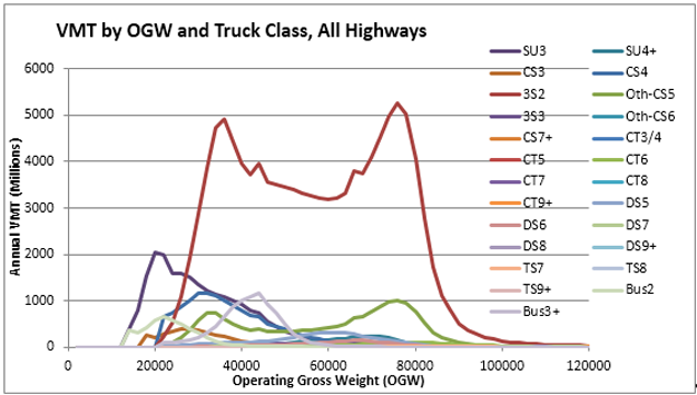
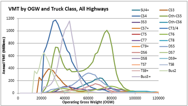
The next graph removes the two most common classes (SU3 and 3-S2) to show the relative importance of the remaining truck classes.
Figure 3 – VMT by OGW and Truck Class, All Highways without SU3 and 3-S2
Axle weight distributions consist of numbers of axle per vehicle falling into each of four axle types (steering axle, single load axle, tandem load axle, and tridem load axle) and 40 weight groups for each type of axle (centered on 1,000-pound categories for single axles, 2,000-pound categories for tandem axles, and 3,000-pound categories for tridem axles). For example, weight group 1 for single axles covers axles from 1 to 1,500 lbs.; group 2 includes axles from 1,501 to 2,500 pounds, and so on. Group 40 includes single axles operating at 39,501 pounds and above. Tandem axle group 1 includes axles from 1 to 3,000 lobs, group 2 axles from 3,001 to 5,000 pounds, etc.
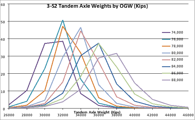
Each OGW of each vehicle class in each region has a unique axle weight and type distribution. Figure 4 below illustrates a sample of tandem axle weight distributions for selected 3-S2 vehicles in one traffic region. Note the range of prevalent axle weights within a given operating weight group—an important factor to consider when evaluating the relative impacts of a particular configuration operating a particular gross vehicle weight.
Figure 4 – 3-S2 Tandem Axle Weights by OGW (Kips)
For use in bridge analysis, all axle weights and types for all vehicle classes are grouped together, and the 12 functional classes are grouped into three highway types for each of two regions. For pavement analysis, the 28 vehicle classes are grouped into 8 classes, and all OGWs in each class are grouped together, and the 12 functional classes are grouped into 3 highway types. Other phases of analysis require other groupings of the data.
previous | next