Comprehensive Truck Size and Weight Limits Study: Pavement Comparative Analysis Technical Report
Chapter 3: Results of Pavement Analysis To Predict Impact of Scenario Traffic
3.1 Impacts of Scenarios on Pavement Performance
The impacts of the six Study scenarios on the performance of the sample pavement sections were assessed by comparison to the base case traffic. Table 8 shows the vehicles that would be allowed under each scenario as well as the current vehicle configuration from which most traffic would likely shift (the control vehicle).
Analysis of Base Case
The pavement analysis averaged the base case (2011) detailed VMT estimates for the States in the vicinity of each geographic location—including estimates of travel by operating gross weight for each vehicle configuration—using the master VMT arrays developed for the study and described the Data Acquisition and Technical Analysis Report. As described in greater detail in that report, separate axle weight and type distributions were developed for each geographic location and for each detailed vehicle class and operating weight group based on data made available by FHWA. Note that a large quantity of WIM data was available, but the available vehicle classification data had significantly less coverage than in previous studies. As a result, estimates of axle weights and types have a higher level of reliability than estimates of VMT by truck configuration, especially for non-Interstate highways.
The USDOT study team compiled and condensed the VMT, operating weight, and axle weight distribution data into the formats needed for input into Pavement ME Design® software (i.e., percentage of truck travel by each summary configuration, number of axles of each type for each summary configuration, and percentage of axles in each of 40 axle weight categories for each type of axle for each summary configuration). Note that the travel and axle distributions vary by geographic location and type of highway (Interstate and other arterial), but not by traffic volume range (HV and MV). Table 3 above depicts trucks per day for each of the volume ranges and highway types in each geographic location.
The default Pavement ME Design® software lane distributions, axle spacings characteristic of each axle type, tire pressures, and truck wheel bases were used. The Pavement ME Design® software was run for each base case traffic level to assess the performance of the pavement sections before any changes in truck size and weight regulations. The results from the base case analyses were found to be reasonable for all of the sample pavement sections. The detailed results for the base case analyses can be found in Appendix K.
Comparison of Base Case and Study Scenario Impacts on Pavement Performance
Each scenario shifted traffic from a base case set of operating weight groups of a small number of vehicle classes to a set of higher operating weight groups. Sometimes the higher operating weight groups were in the same vehicle class and sometimes they were in another vehicle class. Full descriptions of the procedures used in estimating these shifts and the resulting shifts in freight are contained in the Volume II: Modal Shift Comparative Analysis report.
| Scenario | Configuration | Depiction of Vehicle | # Trailers or Semi-trailers | # Axles | Gross Vehicle Weight (pounds) |
Roadway Networks |
|---|---|---|---|---|---|---|
| Control Single | 5-axle vehicle tractor,53 foot semitrailer (3-S2) | 1 | 5 | 80,000 | STAA 1 vehicle; has broad mobility rights on entire Interstate System and National Network including a significant portion of the NHS | |
| 1 | 5-axle vehicle tractor, 53 foot semitrailer (3-S2) | 1 | 5 | 88,000 | Same as Above | |
| 2 | 6-axle vehicle tractor, 53 foot semitrailer (3-S3) | 1 | 6 | 91,000 | Same as Above | |
| 3 | 6-axle vehicle tractor, 53 foot semitrailer (3-S3) | 1 | 6 | 97,000 | Same as Above | |
| Control Double | Tractor plus two 28 or 28 ½ foot trailers (2-S1-2) | 2 | 5 | 80,000 maximum allowable weight 71,700 actual weight used for analysis 2 | Same as Above | |
| 4 | Tractor plus twin 33 foot trailers (2-S1-2) | 2 | 5 | 80,000 | Same as Above | |
| 5 | Tractor plus three 28 or 28 ½ foot trailers (2-S1-2-2) | 3 | 7 | 105,500 | 74,500 mile roadway system made up of the Interstate System, approved routes in 17 western states allowing triples under ISTEA Freeze and certain four-lane PAS roads on east coast 3 | |
| 6 | Tractor plus three 28 or 28 ½ foot trailers (3-S2-2-2) | 3 | 9 | 129,000 | Same as Scenario 5 3 |
1 The network is the 1982 Surface Transportation Assistance Act (STAA) Network (National Network or NN) for the 3-S2, semitrailer (53’), 80,000 pound gross vehicle weight (GVW) and the 2-S1-2, semitrailer/trailer (28.5’), 80,000 pound. GVW vehicles. The alternative truck configurations have the same access off the network as its control vehicle. return to Footnote 1
2 The 80,000 pound weight reflects the applicable Federal gross vehicle weight limit; a 71,700 gross vehicle weight was used in the study based on empirical findings generated through an inspection of the weigh-in-motion data used in the study. return to Footnote 2
3 The triple network starts with the network used in the 2000 Comprehensive Truck Size and Weight (CTSW) Study and overlays the 2004 Western Uniformity Scenario Analysis. The LCV frozen network for triples in the Western States was then added to the network. The triple configurations would not have the same off network access as its control vehicle, the 2-S1-2, semitrailer/trailer (28.5’), 80,000 pound GVW. Use of the triple configurations beyond the triple network would be limited to that necessary to reach terminals that are immediately adjacent to the triple network. It is assumed that the triple configurations would be used in Less-Than-Truck Load (LTL) line-haul operations (terminal to terminal). As a result, the 74,454 mile triple network used in this Study includes: 23,993 mile network in the Western States (per the 2004 Western Uniformity Scenario Analysis, Triple Network), 34,802 miles in the Eastern States, and 15,659 miles in Western States that were not on the 2004 Western Uniformity Scenario Analysis, and the Triple Network used in the 2000 Comprehensive Truck Size and Weight Study (2000 CTSW Study). return to Footnote 3
The characteristic axle weight and type distributions for each vehicle class and operating weight group were applied to the new distribution of vehicle weights and types to derive the traffic input changes needed to apply Pavement ME Design® software to each scenario. Daily traffic volumes were decreased to reflect the smaller number of trucks needed to carry the same amount of freight and adjusted upward to account for the freight diverted from other modes of transportation.
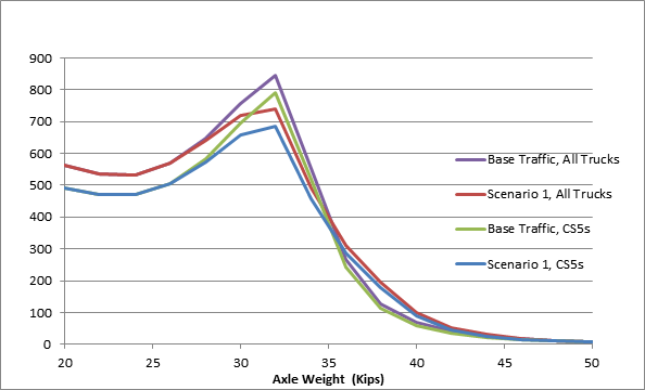
Scenario 1 allows five-axle semitrailer (3-S2) trucks to increase from 80,000 lb. to 88,000 lb. and allows tandem axle weights to increase from 34,000 lb. to 38,000 lb. Since most of these vehicles operate below the current legal maximum weights, the modal shift estimates for this scenario show fairly small upward shifts in operating weights. They also do not show any shifts from other vehicle types to five-axle single-semitrailer combination vehicles. Overall, there is a small upward shift in the distribution of tandem axle weights, both for five-axle conventional semitrailer combinations (3-S2) and for all trucks (see Figure 2, below). Overall the scenario shows a net decrease of 0.6 percent in tandem axles on Interstate highways and a decrease of 0.5 percent on Other NHS highways, (0.2 percent to 0.4 percent) in the number of axle loads.
Figure 2: Scenario 1 Changes in Interstate Tandem Axle Loads
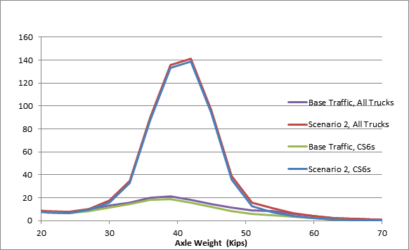
Scenario 2 allows six-axle semitrailer (3-S3) trucks with a tandem drive axle and tridem trailer axle to operate at weights up to 91,000 lb. The scenario also allows tridem axle weights up to 45,000 lb. The modal shift estimates resulted from shifting a portion of five-axle single-semitrailer traffic (3-S2) for operating weights between 76,000 lb. and 90,000 lb. to six-axle vehicles (3-S3) weighing between 80,000 and 91,000 lb., resulting in shifts away from some of the heaviest tandem axle sets to tridem axle sets, as shown in Figure 3 and Figure 4, respectively. Overall, this scenario resulted in reductions in the average number of tandem axles of 4.9 percent on Interstate highways and 4.1 percent on other NHS highways. Single axles decreased by 1.7 percent on Interstate highways and by 1.0 percent on other NHS highways.
Figure 3: Scenario 2 Changes in Interstate Tandem Axle Loads
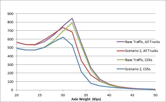
Figure 4: Scenario 2 Changes in Interstate Tridem Axle Loads
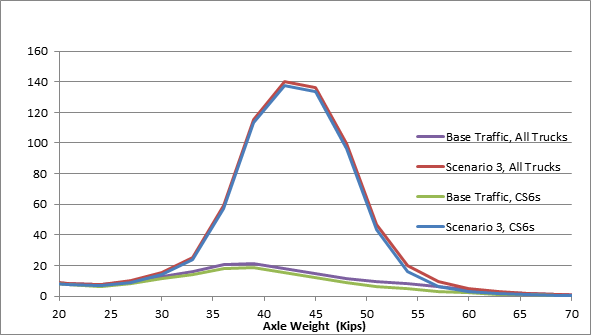
Scenario 3 allows six-axle semitrailer (3-S3) combination trucks with a tandem drive axle and tridem trailer axle to operate at weights up to 97,000 lb. It also allows tridem axle weights up to 51,000 lb. As with Scenario 2, the modal shift estimates considered shifts only from five-axle semitrailer to six-axle semitrailer; in this case, however, there is shifting from five -axle semitrailer traffic (3-S2) for operating weights between 76,000 lb. and 96,000 lb. to six-axle vehicles (3-S3) weighing between 80,000 and 97,000 lb., resulting in even more pronounced shifts away from some of the heaviest tandem axle sets to tridem axle sets, as shown in Figure 5 and Figure 6, respectively. Overall, this scenario resulted in reductions in the average number of tandem axles of 6.7 percent on Interstate highways and 5.6 percent on other NHS highways. Single axles decreased by 2.6 percent on Interstate highways and by 1.5 percent on other NHS highways.
Figure 5: Scenario 3 Changes in Interstate Tandem Axle Loads
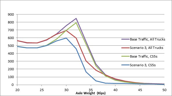
Figure 6: Scenario 3 Changes in Interstate Tridem Axle Loads
Scenario 4 allows trailer lengths on five-axle twin-trailer (2-S1-2) trucks to increase from 28 feet to 33 feet, resulting in significantly higher available cubic capacity. Unlike with Scenarios 1 to 3, which allowed higher operating weights but no increase in trailer volumes, Scenario 4 caters to the large proportion of truck traffic whose capacity is limited by size rather than by weight. The modal shift analysis shows significant shifts from configurations with five-axle single-semitrailer trucks with weights between 40,000 lb. and 70,000 lb. and shorter five-axle twins weighing between 42,000 and 79,000 lb. to configurations featuring longer five-axle twin-trailers weighing between 44,000 and 80,000 lb.
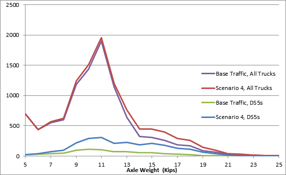
Overall, 10 percent of five-axle single-semitrailer trucks and 72 percent of shorter five-axle twins are projected to shift to heavier and longer five-axle twin-trailers under this scenario, resulting in shifts away from light- and moderate-weight tandem axle sets to higher-range single axles, as shown in Figure 7 and Figure 8, respectively. Overall, this scenario resulted in reductions in the average number of tandem axles of 8.7 percent on Interstate highways and 7.5 percent on other NHS highways. Single axle vehicles increased by 10.2 percent on Interstate highways and by 6.0 percent on other NHS highways.
Figure 7: Scenario 4 Changes in Interstate Tandem Axle Loads
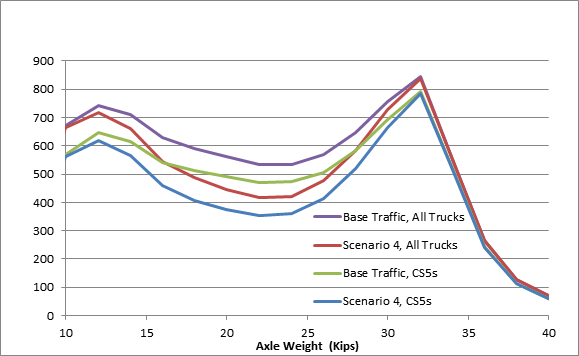
Figure 8: Scenario 4 Changes in Interstate Single Axle Loads
Scenario 5 allows seven-axle triple trailers (2-S1-2-2) that weigh up to 105,000 lb. on a designated highway network that consists of the Interstate system and selected other principal arterials. Since a number of freight destinations are not on the designated network, the modal shift analysis assumed that some portion of most trips would require conversion of two triple-trailer combinations into three twin-trailer combinations when the triple-trailer combination left the designated network. The modal shift analysis shows shifts from five-axle semitrailer trucks with weights between 38,000 lb. and 80,000 lb., and from five-axle twins weighing between 40,000 and 80,000 lb. to seven-axle triple trailers weighing between 54,000 and 105,000 lb. on the designated network and to five-axle twins weighing between 40,000 and 74,000 lb. off the designated network.
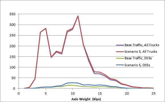
The net effect of the scenario results in fewer lighter and moderate weight tandem axle sets, as shown in Figure 9, with little change to the distribution of single axles on the Interstate system, as shown in Figure 10, but larger shifts to heavier single axles on other NHS highways, as shown in Figure 11. Overall, this scenario resulted in reductions in the average number of tandem axles of 3.4 percent on Interstate highways and 5.8 percent on other NHS highways. Single axles decreased by 2.4 percent on Interstate highways and increased by 2.7 percent on other NHS highways.
Figure 9: Scenario 5 Changes in Interstate Tandem Axle Loads
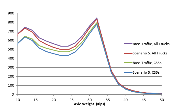
Figure 10: Scenario 5 Changes in Interstate Single Axle Loads
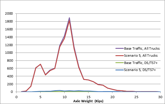
Figure 11: Scenario 5 Changes in Other NHS Single Axle Loads
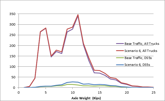
Scenario 6 is very similar to Scenario 5 except that the Scenario 6 triple trailer combination has nine axles (3-S2-2-2) opposed to seven axles for Scenario 5 (2-S1-2-2) and can weigh up to 129,000 lb. as opposed to Scenario 5’s 105,500 gross vehicle weight. Each of these configurations was limited in their travel to a designated network consisting of the Interstate system and access controlled principal arterials. The modal shift analysis assumed that some portion of most trips would require conversion of two triple-trailer combinations into three twin-trailer combinations when the triple-trailer combination left the designated network. The modal shift analysis shows modest shifts from five-axle semitrailer trucks with weights between 38,000 lb. and 80,000 lb. and from five-axle twins weighing between 40,000 and 80,000 lb. to nine-axle triple trailers weighing between 56,000 and 129,000 lb. on the designated network. The shift can also occur to five-axle twins weighing between 40,000 and 86,000 lb. off of the designated the network.
As with Scenario 5, the net effect of the scenario results in fewer light- and moderate- weight tandem axle sets, as shown in Figure 12, with little change to the distribution of single axles on the Interstate system, as shown in Figure 13, but larger shifts to heavier single axles on other NHS highways, as shown in Figure 14. Overall, this scenario resulted in reductions in the average number of tandem axles of 0.4 percent on Interstate highways and 3.7 percent on other NHS highways. Single axles increased by 2.1 percent on Interstate highways and by 4.6 percent on other NHS highways.
Figure 12: Scenario 6 Interstate Tandem Axle Weight Loads
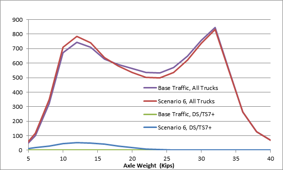
Figure 13: Scenario 6 Interstate Single Axle Weight Loads
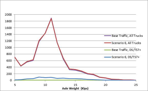
Figure 14: Scenario 6 Changes in Other NHS Single Axle Loads
The impacts of the six scenarios on the structural performance of the sample pavement sections were assessed by comparing the changes in predicted initial service intervals at the specified reliability level. The approach used the Pavement ME Design® software to provide performance predictions for each scenario as compared with the base case predicted performance. The initial service interval for each case was identified based on the distress thresholds presented in Table 4. The detailed result tables are presented in Appendix L for all of the sample pavement sections. A predicted pavement life factor, defined as the time to first rehabilitation for the scenario divided by the time to first rehabilitation for the base case, was computed for each pavement type in each geographic location to facilitate assessing the impacts of each scenario on pavement costs. Since the base case was considered the baseline for each pavement type in each geographic location, it was assigned a predicted pavement life factor of 1.0. The performance associated with the six scenarios was then compared to the performance of the baseline to compute predicted life factors for each.
Rehabilitation Treatment Type and Frequency of Application
The most common type of rehabilitation treatment for cracking in both flexible and rigid pavements is the placement of an asphalt overlay. The asphalt overlay thicknesses used for application to existing flexible and rigid pavement types for the pavement life cycle cost analysis are presented in Table 9.
The rehabilitation treatment types selected for the next step in the analysis were based on the failure mechanisms predicted in the pavement performance analysis. The failures predicted for rigid pavements were either by transversely cracked slabs, faulting, or roughness (IRI), while the failures predicted for flexible pavements were by rutting, IRI, or fatigue cracking. The issues with faulting or IRI in concrete pavements can be addressed by diamond grinding the surface for a number of years, but ultimately may require a structural overlay.
The existing pavement rehabilitation treatment survival analyses was used as a basis to determine the appropriate treatment frequency of diamond grinding and asphalt overlay placement for this study. The mean life for rigid pavement diamond grinding was reported to range from 14.0 years (Darter and Hall, 1990) to 16.8 years (California Department of Transportation, 2007). A survival analysis study on both flexible and rigid pavements in Utah reported that the mean life for asphalt overlay treatments was 12 years (Hoerner et al., 1999). Therefore, the treatment type and frequency of application over a 50-year performance period were selected and are presented in Table 10 for both flexible and rigid pavements. Note that the thickness of the asphalt overlay varies depending on the facility type (Interstate versus other NHS, but the timing of application was consistent).
Within the frame of a fifty year life cycle, the algorithm applied for flexible pavement rehabilitation was to first mill and apply a structural AC overlay assumed to last 12 years. After 12 years, another mill and slightly thinner AC overlay would be placed and again assumed to last for 12 years. The process would be repeated a third time, and then, after the third 12 year overlay life span ended, the road would be fully reconstructed.
Again, within the frame of a fifty year life cycle, the algorithm applied for rigid pavement rehabilitation depended on the primary distress type. If the pavement failed in slab cracking, a structural AC overlay was placed over the existing concrete and assumed to last 12 years. After 12 years, a thinner AC overlay would be placed and again assumed to last for 12 years. The process would be repeated a third time, but after the third overlay’s 12 year life span, a full reconstruction of the entire overlaid concrete pavement would be implemented.
If the rigid pavement failed in faulting or IRI, the pavement surface was diamond ground and the resulting ride quality was assumed to last for 15 years. The same process and timing would be repeated three times, followed by a structural AC overlay.
The treatment strategies presented in Table 10 were carried forward to assess the impacts of the scenarios on pavement costs.
3.2 References
California Department of Transportation, "Chapter 5 Diamond Grinding and Grooving," MTAG Volume II - Rigid Pavement Preservation 2nd Edition, California Division of Maintenance, 2007.
Darter, M., and K. Hall, “Performance of Diamond Grinding,” Transportation Research Record No. 1268, Transportation Research Board, National Research Council, Washington, D.C., 1990.
Hoerner, T., Darter, M., Gharaibeh, N., and T. Crow, “Comparative Performance and Costs of In-service Highway Pavements, I-15 Utah”, Technical Report, ERES Consultants, Inc., 1999.
You may need the Adobe® Reader® to view the PDFs on this page.
previous | next