4. Proposed Framework
Based on the previous discussion, this section addresses the general micro-economic framework in both geometric as well as mathematical terms. The framework is general in the sense that it captures benefits of any highway improvement[16]. The introduction of ITS, for instance, to manage congestion would translate into reduced travel times and enhancing reliability. Benefits of any initiative affecting overall logistics costs – such as vehicle operating limits – could be considered. An explanation of key parameters within the framework will be given so as to build a practical cost-benefit model.
4.1 Approach
Recall that in NCHRP 2-17(4) [2], a method was developed to estimate the elasticity of logistics cost with respect to travel time savings, call it![]() η × C/T. This quantity was derived from a sample of firms response (cost savings) to travel time improvements. A similar approach can be used to determine a firm's elasticity of demand for transportation as a result of travel time savings and changes in logistics, call this elasticity
η × C/T. This quantity was derived from a sample of firms response (cost savings) to travel time improvements. A similar approach can be used to determine a firm's elasticity of demand for transportation as a result of travel time savings and changes in logistics, call this elasticity![]() η × VM/T. This last quantity encapsulates the firm's response to highway improvements in terms of new transportation demand as a result of possible substitutions. The quantity is shown graphically below over a sample of several firms. The points at which re-organization occurs,
η × VM/T. This last quantity encapsulates the firm's response to highway improvements in terms of new transportation demand as a result of possible substitutions. The quantity is shown graphically below over a sample of several firms. The points at which re-organization occurs,![]() W1, may be specific to individual firms. The trend will allow the inference of effects (slope of the curve) over a range of firms.
W1, may be specific to individual firms. The trend will allow the inference of effects (slope of the curve) over a range of firms.
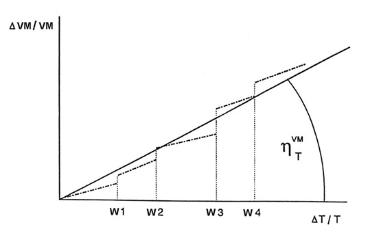
Exhibit 23: Aggregate relative change in transportation demand with respect to relative travel time savings.
According to 3.6, to calculate benefits of road improvements, the elasticity of transportation demand with respect to transportation cost ![]() η × VM/C is required. A simple relationship can be established between these two elements. We can write
η × VM/C is required. A simple relationship can be established between these two elements. We can write![]() η × VM/C as:
η × VM/C as:
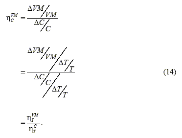
This last expression is the ratio of the elasticity of transport demand with respect to travel time![]() η × VM/T, and the elasticity of transportation cost with respect to travel time
η × VM/T, and the elasticity of transportation cost with respect to travel time![]() η × C/T. Both of these might be estimated using a suitable sampling methodology within various industries.
η × C/T. Both of these might be estimated using a suitable sampling methodology within various industries.
Central to the framework, increases in transport demand are needed as a result of infrastructure improvements. It is acknowledged that the elasticity of vehicle miles may be difficult to obtain. Options may include simulation, or a generalized demand function.
There is one modification that must be brought to the approach. While the units for C were previously logistics costs, the new units will be logistics cost per unit of transportation (vehicle-mile, product-mile, ton-mile etc). This change of scale will allow the integration of the demand curve into net benefits. Estimation of transportation user costs should not present a problem. For instance, assuming for the sake of argument that wages accounted for 30% of transport operating [9], a 20% decrease in travel time could result in a 6% decrease of direct transportation cost per vehicle mile. In reality, other substitutions could also take place.
This approach has the added advantage that the demand for transportation services can be aggregated across markets or commodities thereby facilitating benefits estimation for highway network improvements. Aggregation using a product demand curve may be difficult due to the varying nature of products. We now turn to the problem of changes in product demand.
The fundamental determination of the demand curve for transportation services involves two quantities, price and vehicle miles used or traveled. The change in each of these components was derived as a function of some third dimension – travel time and/or travel time variability. This third dimension is in turn a function of highway investment. Once time savings are known or estimated, logistics cost savings estimation can be carried out at the level of the firm to include logistics re-organization effects. Each firm is different, but with a representative sample the general response trend can be quantified over specific industries. Note that the third dimension could also include changes in vehicle capacity or service hours thereby increasing freight throughput. Whatever effect is considered, it is the net change in generalized logistics cost per vehicle mile that must be estimated.
Changes in Output/Product Demand
The demand for freight services is derived from the demand for final products carried. Because freight transport is closely related to land use patterns, it is also important to consider at the same time influences affecting industrial location and distribution. Transport demand could thus increase due to two effects – both of which have been mapped at Exhibit 22. First, logistics re-organization may result in substitution of additional transport for inventory and holding locations. Second, savings from lower transportation and overall logistics costs may be passed on to consumers resulting in an increase of consumer product demand. This increase in demand is embodied in increases in transportation services required. Both these components must be part of the effective demand upon which net benefits are derived.
4.2 Competitive Market
The benefits of infrastructure investment can be derived from the change in consumer surplus for transportation demand. In general form, it is possible to write:
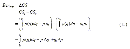
In our case, price![]() p(q) = C(VM) the cost of transport per vehicle mile at a level of demand
p(q) = C(VM) the cost of transport per vehicle mile at a level of demand![]() q = VM. This general expression encapsulates the net benefit of the infrastructure improvement in the absence of marginal cost pricing.
q = VM. This general expression encapsulates the net benefit of the infrastructure improvement in the absence of marginal cost pricing.
One approach to evaluating the integral above would be to assume constant elasticity of demand near the present demand level. A general expression for a constant-elasticity-of-demand schedule is![]() Q = a/Pb where Q is the quantity that would be sold at a price of P and where a and b are constants. It is a simple matter to evaluate the integral.
Q = a/Pb where Q is the quantity that would be sold at a price of P and where a and b are constants. It is a simple matter to evaluate the integral.

The next section shows the derivation for a linear case as was done in NCHRP 342.
4.2.1 Special Case – Linear Demand Curve
If![]() q1 is much larger than
q1 is much larger than![]() q0 and/or the demand curve is highly concave, then the shape of the demand curve may have an effect on benefits estimation. If
q0 and/or the demand curve is highly concave, then the shape of the demand curve may have an effect on benefits estimation. If![]() q0 is approximately equal to
q0 is approximately equal to![]() q1 and the demand curve
q1 and the demand curve![]() p(q) is well behaved, then a linear approximation may be adequate.
p(q) is well behaved, then a linear approximation may be adequate.
For the simple case of a linear demand curve,![]() C = a − bVM. For this case, it is possible to show that:
C = a − bVM. For this case, it is possible to show that:

where![]() a = (C0 + C0/η × VM/C) and
a = (C0 + C0/η × VM/C) and![]() b = (C0/η × VM/C × VM0).
b = (C0/η × VM/C × VM0).
The change in transportation cost can be estimated as:

We can therefore derive the new price![]() p1 as:
p1 as:
where![]() ε is the fraction of the per mile cost savings transferred to customers.
ε is the fraction of the per mile cost savings transferred to customers.
The change in demand can be estimated as:

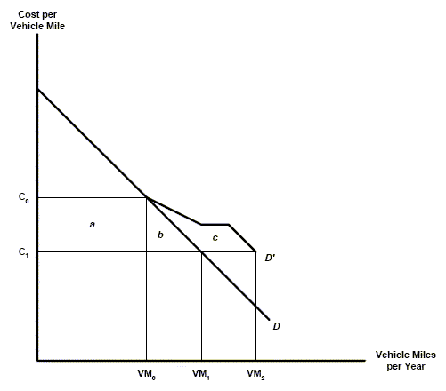
Exhibit 24: Demand curve for transportation.
Net benefits are represented by areas a, b, and c, the direct benefit, the medium and long run demand changes respectively. Instead of a uniform shift in the demand curve, there is an extension of demand made possible by re-organization, product price reductions, and increased product demand. With this approach, it is possible to estimate total benefits with and without re-organization as was done in NCHRP 2-17(4). The great advantage of using a simple demand curve is that it includes all benefits.
4.3 Monopoly
For the case of monopoly, it was shown that net benefits involve both a consumer's gain as well as a producer's gain. This is true not just for transportation, but also for other markets.
The consumers gain![]() ∆CS is as above. The producer's gain
∆CS is as above. The producer's gain![]() ∆CS′ has the exact same form except that the price is replaced by marginal revenue
∆CS′ has the exact same form except that the price is replaced by marginal revenue![]() ∂R/∂q. The new price that maximizes the monopolist's profit can be approximated as
∂R/∂q. The new price that maximizes the monopolist's profit can be approximated as![]() B = A − ∆CLog. These two areas are illustrated graphically below. In the case of monopoly, two areas must be considered, but the overall procedure for each is the same. The expression is:
B = A − ∆CLog. These two areas are illustrated graphically below. In the case of monopoly, two areas must be considered, but the overall procedure for each is the same. The expression is:

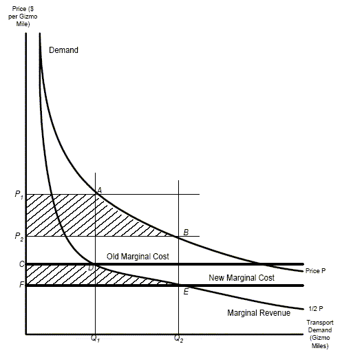
Exhibit 25: Benefits in the presence of Monopoly
4.4 Accounting for Non-Marginal Cost Pricing
A simple adaptation of the cost-benefit methodology can be used to correct for non-marginal cost pricing. If TC is the total cost of providing a road with N trips made along it per unit time, then this total cost can be defined as:
where C is the cost of one trip to a vehicle and![]() f(K) is the cost per time period of providing K units of road capacity. The short-term marginal cost becomes:
f(K) is the cost per time period of providing K units of road capacity. The short-term marginal cost becomes:

The Nth vehicle then incurs a cost itself and imposes a cost on other users. This is demonstrated graphically at Exhibit 26 below.
The cost-benefit analysis could be revised with estimated marginal social cost prices for the use of transport services – at a given level of use. These estimated price adjustments could have a wide margin of uncertainty. However, if a highway improvement option remains justified and highly ranked compared to other competing alternatives in the presence of approximate marginal cost pricing, then there is good confidence that the option valuations are robust to underlying assumptions. The actual estimation of marginal cost prices is work to be carried out as part of a follow-on task.
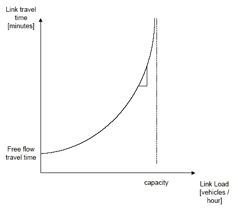
Exhibit 26: Typical user link travel time graph and marginal cost.
4.5 Approach Summary
In summary, our method rests on estimating the change in consumer surplus reflected in the 'shift' in the demand curve for freight transport that follows the improvement. This was the general idea presented in Appendix D of 342, but significant changes are made (aside from resolving the mathematical problems we found): the 'shift' in the demand curve now reflects increasing output as well as trade-offs between transportation spending and total logistics costs. We have thus moved away from the "simplified approach" presented at the end of Appendix D.
From a theoretical standpoint, we could stop here but we now turn to implementation. One possibility for empirical estimation of the demand curve is to use elasticity estimates of the type developed in 2-17(4). These elasticities embody increases in output as well as substitution of transportation for inventory-holding points. Corrections have been proposed for monopoly and marginal-cost pricing.
previous | next