3. Empirical Results
3.1 Estimating Regional Elasticities of Demand
Chapter 2 described tests employed to select a geographic division. Based on the tests and empirical results achieved, the project team selected an approach for estimating the elasticity of demand with respect to highway performance. This section describes and reports the results obtained.
The following equation was estimated separately for each region (East, Central, and West), when demand for daily truck traffic is specified as a function of delay and real per capita income growth:
Log(AADTTc,t) = βc + β1Delayc,t + β2Incomec,t
where:
AADTT = Average annual daily truck traffic
Delay = Average delay per mile
Income = Real per capita income growth
t = 1993, 1994,… 2003
c = Corridor
![]() βc
are corridor-specific constant, or fixed effects, where:
βc
are corridor-specific constant, or fixed effects, where:
c = 1,…, 16 for East,
c = 1,…, 18 for Central,
c = 1,…, 21 for West
The coefficient![]() β1 from the log-lin specification of the model above might be transformed into the elasticity coefficient. In calculus notation,
β1 from the log-lin specification of the model above might be transformed into the elasticity coefficient. In calculus notation,![]() β1 can be expressed as
β1 can be expressed as
,
And since the elasticity coefficient (elasticity of demand with respect to highway performance-delay) is defined as
,
Therefore
.
The regression results are summarized in Tables 16, 17, and 18 for the East, Central, and West regions, respectively. The models explain a high percentage of variability in freight demand measured by average annual daily truck traffic, at about 79% for the East, 95% for the Central, and about 94% for the West.
The coefficients on the delay and income variable have the correct signs and are statistically significant. The only exception is the coefficient on income in the model for the West region (see Table 18), which is insignificant at the 5% level. However, it is significant at the 10% level.
| Dependent Variable: LOG(AADTT) | ||||
|---|---|---|---|---|
| Method: Pooled EGLS (Cross-section weights) | ||||
| Total pool (unbalanced) observations: 114 | ||||
| Variable | Coefficient | Std. Error | t-Statistic | p-value |
| Constant | 8.847002 | 0.013168 | 671.8803 | 0.0000 |
| Delay | -0.005117 | 0.002344 | -2.182555 | 0.0315 |
| Real Per Capita Income Growth | 0.008595 | 0.004069 | 2.112079 | 0.0373 |
| Fixed Effects: | ||||
| Atlanta-Jacksonville | 0.125424 | |||
| Atlanta-Knoxville | 0.323139 | |||
| Atlanta-Mobile | -0.233984 | |||
| Birmingham-Nashville | -0.232907 | |||
| Columbus-Pittsburgh | -0.054241 | |||
| Harrisburg-Philadelphia | 0.012104 | |||
| Mobile-New Orleans | -0.259956 | |||
| Richmond-Philadelphia | 0.44495 | |||
| Boston-New York City | 0.032609 | |||
| Harrisburg-New York City | 0.154785 | |||
| Detroit-Pittsburgh | -0.104274 | |||
| Philadelphia-New York City | -0.106916 | |||
| New York City-Cleveland | 0.037953 | |||
| Miami-Richmond | -0.261302 | |||
| Miami-Atlanta | -0.176157 | |||
| Knoxville-Harrisburg | 0.297654 | |||
| R-squared | 0.78757 | Mean dependent var | 8.856317 | |
| Sum squared resid | 1.534467 | Durbin-Watson stat | 1.020177 | |
| Dependent Variable: LOG(AADTT) | ||||
|---|---|---|---|---|
| Method: Pooled EGLS (Cross-section weights) | ||||
| Total pool (unbalanced) observations: 138 | ||||
| Variable | Coefficient | Std. Error | t-Statistic | p-value |
| Constant | 8.745927 | 0.011244 | 777.8526 | 0.0000 |
| Delay | -0.069076 | 0.019921 | -3.467458 | 0.0007 |
| Real Per Capita Income Growth | 0.00866 | 0.003502 | 2.473205 | 0.0148 |
| Fixed Effects: | ||||
| Cleveland-Columbus | 0.187098 | |||
| Dayton-Detroit | 0.127923 | |||
| Indianapolis-Chicago | 0.176353 | |||
| Indianapolis-Columbus | 0.345631 | |||
| Kansas City-St Louis | 0.192902 | |||
| Knoxville-Dayton | 0.322572 | |||
| Louisville-Columbus | 0.231423 | |||
| Louisville-Indianapolis | 0.198499 | |||
| Nashville-Louisville | 0.598196 | |||
| Nashville-St Louis | -0.398262 | |||
| St Louis-Indianapolis | 0.189179 | |||
| Omaha-Chicago | 0.01184 | |||
| Chicago-Cleveland | -0.206494 | |||
| Billings-Sioux Falls | -1.651534 | |||
| Amarillo-Oklahoma City | 0.142811 | |||
| Memphis-Dallas | 0.373809 | |||
| Memphis-Oklahoma City | 0.165234 | |||
| St Louis-Oklahoma City | -0.349393 | |||
| R-squared | 0.948179 | Mean dependent var | 8.744014 | |
| Sum squared resid | 2.002249 | Durbin-Watson stat | 1.010586 | |
| Dependent Variable: LOG(AADTT) | ||||
|---|---|---|---|---|
| Method: Pooled EGLS (Cross-section weights) | ||||
| Total pool (unbalanced) observations: 129 | ||||
| Variable | Coefficient | Std. Error | t-Statistic | p-value |
| Constant | 8.370945 | 0.011247 | 744.2735 | 0.0000 |
| Delay | -0.015586 | 0.00573 | -2.720287 | 0.0076 |
| Real Per Capita Income Growth | 0.005534 | 0.003323 | 1.665585 | 0.0987 |
| Fixed Effects: | ||||
| Dallas-Houston | 0.533012 | |||
| San Antonio-Houston | 0.335623 | |||
| Denver-Kansas City | -0.672123 | |||
| Denver-Salt Lake City | 0.044107 | |||
| San Francisco-Salt Lake City | -0.632347 | |||
| San Francisco-Los Angeles | 0.247815 | |||
| Portland-Seattle | 0.668379 | |||
| San Diego-Los Angeles | 0.544992 | |||
| Seattle-Billings | -0.6264 | |||
| Seattle-Sioux Falls | -0.867802 | |||
| Portland-Salt Lake City | -0.276968 | |||
| Los Angeles-Tucson | 0.097899 | |||
| Tucson-San Antonio | 0.557139 | |||
| Laredo-San Antonio | -0.06466 | |||
| Nogales-Tucson | 0.28696 | |||
| San Antonio-Dallas | 0.669072 | |||
| Barstow-Bakersfield | 0.257096 | |||
| Barstow-Amarillo | 0.105583 | |||
| Barstow-Salt Lake City | -0.156777 | |||
| Galveston-Dallas | 0.343733 | |||
| Dallas-El Paso | 0.198615 | |||
| R-squared | 0.940778 | Mean dependent var | 8.377655 | |
| Sum squared resid | 1.913074 | Durbin-Watson stat | 0.776213 | |
The semi-logarithmic functional form of the estimated equations requires the coefficients on the delay variable to be transformed in order to interpret them in elasticity terms. Table 19 shows this step and provides a summary of findings regarding the impact of changes in delay on freight demand.
| Region | Coefficient on Delay | Implied Elasticity | Interpretation |
|---|---|---|---|
| East | -0.005117 | -0.0076 | Other things being equal, a 10% increase in delay per mile reduces freight demand by 0.07%. |
| Central | -0.069076 | -0.0175 | Other things being equal, a 10% increase in delay per mile reduces freight demand by 0.175%. |
| West | -0.015586 | -0.0070 | Other things being equal, a 10% increase in delay per mile reduces freight demand by 0.07%. |
3.2 Calculating Regional Additive Freight Reorganization Benefits
3.2.1 Microeconomic Framework
Figure 4 gives a diagrammatic representation of the microeconomic framework which identifies the benefits of industrial reorganization. Area A represents the immediate benefits of a highway improvement to existing highway users (principally user time savings and reduced vehicle operating costs). Area B represents the immediate benefits accruing to users newly attracted to the highway by virtue of the improvement. Areas A and B together represent the benefits conventionally measured in a CBA.
Area C represents the value of efficiency gains to the economy due to industrial reorganization precipitated by the highway improvement. Industrial reorganization means the adoption of advanced logistics the firm's business case for which depend on the likelihood of a threshold level of reliability in highway performance. Defined as the ratio of area C to the sum of areas A and B namely,![]() C/[A+B] expressed as a percentage, the "additive freight reorganization benefit" gives the percentage by which to increase the value of conventionally-measured benefits to freight traffic in order to approximate total benefits. In other words, the benefits inclusive of the reorganization effect.
C/[A+B] expressed as a percentage, the "additive freight reorganization benefit" gives the percentage by which to increase the value of conventionally-measured benefits to freight traffic in order to approximate total benefits. In other words, the benefits inclusive of the reorganization effect.
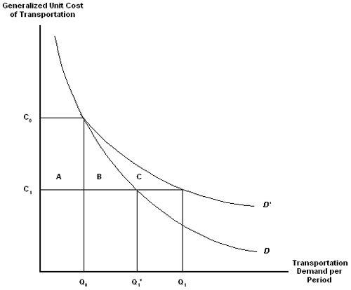
Figure 4. Change in Consumer Surplus from Changing Demand for Transportation as a Function of Unit Generalized Transportation Cost
To assess the quantitative significance of the additive reorganization benefit, the study amassed quantitative evidence of the following:
As discussed in the Phase II report on the national analysis, a variable-elasticity form of the present and post-reorganization demand curves (indicating constant returns to scale) provides a reasonable description of the available data. Specifically, the elasticity of demand for transport with respect to generalized cost is found to vary proportionately with generalized cost. This means that the elasticity is smaller when generalized cost is relatively low, and it is higher when generalized cost is relatively high, implying that demand is more sensitive to changes in highway conditions when congestion is high than when congestion is low. The form of the estimated demand curve is:
where Q is the quantity of transportation that would be demanded at a generalized cost of C, and where![]() β0 and
β0 and![]() β1 are constants estimates with least-squares in a fixed-effects model that controls for between-corridor variations.
β1 are constants estimates with least-squares in a fixed-effects model that controls for between-corridor variations.
3.2.2 Additive Benefit Calculation Module
The additive benefit estimation module has been developed to accommodate outcomes from two broad categories of cost benefit analysis models: 1) standard user cost models, where the practitioner focuses on the reduction of user costs to existing highway users (baseline transportation demand, as measured by truck vehicle miles traveled (VMT) or other metrics) and ignore induced demand (additional highway trips brought about by the reduction in transport costs); and 2) consumer surplus models, where the practitioner explicitly accounts for induced demand using standard transportation demand elasticity estimates and estimates the change in consumer surplus resulting from a candidate highway investment.
Additive Benefit Estimation with Standard User Cost Models
In Figure 5, the additive benefit would be estimated as the ratio of indirect benefits, represented by the red triangle B (the area between the long run transport demand curve and the![]() C1 line, and bounded by
C1 line, and bounded by![]() VM0 and
VM0 and![]() VM1), to direct benefits, represented by the blue rectangle A (the area between the
VM1), to direct benefits, represented by the blue rectangle A (the area between the![]() C0 and
C0 and![]() C1 lines and to the left of
C1 lines and to the left of![]() VM0).
VM0).
With the application of the additive benefit factor, direct benefits (or benefits to existing highway users) are augmented to represent total benefits (direct plus indirect benefits). Total benefits within this framework are measured by the change in consumer surplus using the long-run demand curve for freight.
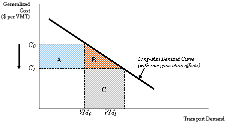
Figure 5. Additive Benefit Estimation with Standard User Cost Models, An Illustration
A numerical example of additive freight reorganization benefit estimation is provided in Table 20.
| # | Parameters | Value | Comments |
|---|---|---|---|
| Unit Generalized Costs ($/vehicle mile) | |||
| 1 | $3.8100 | Assumption / input. | |
| 2 | $3.4351 | Assumption (10% reduction). | |
| Transport Demand (freight vehicle miles) | |||
| 3 | 200,000 | Assumption / input. | |
| 4 | 220,434* | Calculated using the nominal elasticity (b). | |
| Demand Curve | |||
| 5 | Constant |
49,879 | |
| 6 | Full Price Elasticity (b) | -1.0382* | |
| 7 | 1.9632 | Estimation of area below demand curve and between |
|
| 8 | 2.98484E-05 | ||
| 9 | 81,679 | ||
| 10 | 70,191 | Estimation of area D. | |
| 11 | 74,988 | Estimation of area A. | |
| 12 | Direct Benefits (Row 11) | $74,988 | User cost savings. |
| 13 | Indirect Benefits (Row 9 minus Row 10) | $11,487 | Estimation of area B (triangle). |
| 14 | Total benefits (Row 12 + Row 13) | $86,476 | Area A + B. |
| 15 | % Indirect / Direct | 15.3%* | The additive benefit factor. |
*Numbers in red signify key variables that illustrate the change in demand.
The full price elasticity (b) on row 6 is estimated by considering the combined impact of the elasticity of demand with respect to out-of-pocket costs (direct vehicle operating costs or shipping rate) and a measure of the long-run elasticity of demand with respect to highway performance (transit time and reliability).
For the purpose of this study, the elasticity of freight demand with respect to transportation costs was derived from the literature (-0.97, Tae Oum). The long-run elasticity of demand with respect to highway performance was estimated econometrically, as part of Phase II and Phase III of the study.
Additive Benefit Estimation with Consumer Surplus Models
In Figure 6, the additive benefit factor would be calculated as the ratio of area F (the area between the long-run transport demand curve "with reorganization effects," the standard short run demand curve, and the![]() C1 line) to a standard measure of consumer surplus, represented by area A plus area E.
C1 line) to a standard measure of consumer surplus, represented by area A plus area E.
In other words, the additive benefit factor is estimated as the percentage change in consumer surplus resulting from incremental transport demand along the long-run demand curve. Incremental transport demand is illustrated by the shift from![]() VM1 to
VM1 to![]() VM2 on Figure 6.
VM2 on Figure 6.
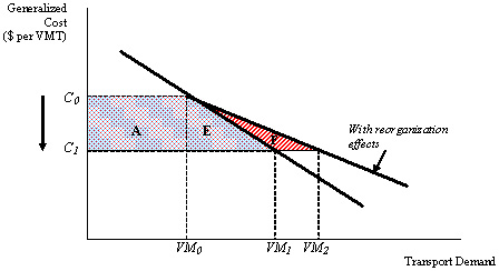
Figure 6. Additive Benefit Estimation with Consumer Surplus Models, An Illustration
A numerical example of additive benefit estimation with consumer surplus models is provided in Table 21.
| # | Parameters | Standard Consumer Surplus Model Output | Augmented Output and Additive Benefit Estimation |
|---|---|---|---|
| Unit Generalized Costs ($/vehicle mile) | |||
| 1 | $3.8100 | $3.8100 | |
| 2 | $3.4351 | $3.4351 | |
| Transport Demand (freight vehicle miles) | |||
| 3 | 200,000 | 200,000 | |
| 4 | 219,400* | 220,434* | |
| Demand Curve | |||
| 5 | Constant |
54,642 | 49,879 |
| 6 | Full Price Elasticity (b) | -0.9700* | -1.0382* |
| 7 | 2.0309 | 1.9632 | |
| 8 | 1.30602E-05 | 2.98484E-05 | |
| 9 | 77,614 | 81,679 | |
| 10 | 66,641 | 70,191 | |
| 11 | 74,988 | 74,988 | |
| 12 | Direct Benefits (Row 11) | $74,988 | $74,988 |
| 13 | Indirect Benefits (Row 9 minus Row 10) | $10,973 | $11,487 |
| 14 | Total benefits (Row 12 + Row 13) | $85,962 | $86,476 |
| 15 | % change in "total benefits" | 0.60%* | |
| 16 | % change in "indirect benefits" | 4.7%* | |
*Numbers in red signify key variables that illustrate the change in demand.
Discussion
Both approaches may be developed for the Phase III tool so that analysts not estimating user costs prior to calculator use would still be able to calculate an additive freight reorganization benefit factor. A review of current CBA approaches suggests that most analysts would likely use the Consumer Surplus approach.
In both models, the calculation is sensitive to the difference between current and anticipated demand (AADTT) and user costs, which are items that will vary project to project. It is proposed that the model also calculate the transformation of the elasticity on a project-by-project basis, factoring in the existing delay on the segment being improved. This would also add variability and local specificity to the additive benefit calculation.
Both approaches will be further assessed and refined as part of Phase III-B.
3.2.3 Regional Additive Benefit Factors
The process of computing the additive benefit factor, explained above, was then applied to the three regions of interest. Each region is defined by its elasticities of demand with respect to performance and price.
Table 22 shows the regional elasticities of demand with respect to highway performance estimated through regression analysis in earlier steps.
| Region | Implied Elasticity |
|---|---|
| East | -0.0076 |
| Central | -0.0175 |
| West | -0.007 |
Several difficulties were encountered in Phase II for the development of price elasticity. Both price and demand elasticity are required for the estimation of an additive benefit factor. One acknowledged and accepted value for price elasticity (derived from estimates by Tae Oum in a national analysis is currently used for each of the three corridors. Therefore the value of -.97, as estimated by Tae Oum, is used here. However, an attempt was made to regionalize this value as follows:
| U.S. | Regional Differences* When Compared to the National Level (-0.97 = 100%) | Regional Estimate of Elasticity of Demand with Regard to Price | ||
|---|---|---|---|---|
| East | 115.3% | East | -1.12 | |
| -0.97 | Central | 99.6% | Central | -0.97 |
| West | 86.9% | West | -0.84 | |
*Note: The regional differences were derived using a proxy variable for which regional data were available. The proxy variable, in this case, is the average V/C ratio. Relating the V/C ratio to the elasticity of demand with respect to price is based upon two assumptions:
- The high level of congestion is an indicator of high-level economic activity.
- The demand for transportation with respect to price is more elastic in areas with a higher-level economic activity.
Using the two elasticities presented above and the computer model described above, sample regional additive benefit factors were calculated, as shown in Table 24. These represent an additive benefit factor for the typical corridor in each regional sample and are provided as an illustration of the additional freight benefits would have been for the average corridor in each region.
Each corridor developing a logistics benefit estimation will derive a unique additive benefit factor based on certain regional and national characteristics:
- Regional elasticity
- Price elasticity
And certain corridor-specific characteristics:
- AADTT
- Delay
- Predicted traffic demand
- User costs
- Calculated freight benefits
| Region | East | Central | West |
|---|---|---|---|
| Additive Benefit Factor | 16.7% | 14.8% | 12.7% |
3.2.4 Commodity Flow Data Analysis
Analysis of FAF commodity flow data was conducted for the East, Central, and West regions. Data available included top commodities by volume (weight) and by value. The data describe regional mixes of freight movement that are similar but not the same.
From a value perspective, finished and semi-finished goods rank high in the mix of goods in each region; however, the specific goods vary by region. Except for the Central region, finished goods were not significant contributors of freight volume. In the Central region, machinery and motorized vehicles were the ninth and tenth largest categories of shipment by volume.
Tables 25 and 26 present the top commodities by thousand tons and dollar value. This greater than average volume of finished and semi-finished goods in the Central region may explain the higher than average elasticity of demand with respect to highway performance in the region.
| Region | Commodity | Thousand Tons |
|---|---|---|
| East | Gravel | 7,173.3 |
| Waste/scrap | 5,999.1 | |
| Cereal grains | 5,110.0 | |
| Other foodstuffs | 4,083.3 | |
| Unknown | 3,956.9 | |
| Nonmetal mineral products | 3,576.3 | |
| Wood prods. | 3,154.3 | |
| Mixed freight | 3,024.1 | |
| Base metals | 2,916.3 | |
| Nonmetallic minerals | 2,322.5 | |
| Central | Base metals | 2,866.0 |
| Nonmetal mineral products | 2,480.8 | |
| Gasoline | 2,013.9 | |
| Other foodstuffs | 1,795.7 | |
| Mixed freight | 1,621.7 | |
| Unknown | 1,587.5 | |
| Waste/scrap | 1,471.8 | |
| Gravel | 1,385.6 | |
| Machinery | 1,164.6 | |
| Motorized vehicles | 1,115.2 | |
| West | Nonmetal mineral products | 14,739.6 |
| Gravel | 7,703.2 | |
| Gasoline | 7,593.5 | |
| Coal, n.e.c. | 4,344.5 | |
| Mixed freight | 3,707.7 | |
| Other foodstuffs | 3,488.1 | |
| Unknown | 3,415.4 | |
| Wood prods. | 3,136.2 | |
| Natural sands | 2,623.0 | |
| Waste/scrap | 2,491.3 |
| Region | Commodity | $M |
|---|---|---|
| East | Mixed freight | 11,824 |
| Machinery | 10,247 | |
| Motorized vehicles | 6,054 | |
| Textiles/leather | 5,047 | |
| Pharmaceuticals | 4,891 | |
| Other foodstuffs | 4,399 | |
| Electronics | 3,951 | |
| Printed prods. | 3,788 | |
| Unknown | 3,690 | |
| Misc. manufacturing products | 3,457 | |
| Central | Machinery | 7,420 |
| Mixed freight | 6,568 | |
| Motorized vehicles | 5,306 | |
| Base metals | 2,672 | |
| Pharmaceuticals | 2,618 | |
| Electronics | 2,159 | |
| Articles-base metal | 1,907 | |
| Misc. manufacturing products | 1,877 | |
| Other foodstuffs | 1,826 | |
| Plastics/rubber | 1,623 | |
| West | Mixed freight | 17,672 |
| Machinery | 13,279 | |
| Electronics | 13,224 | |
| Motorized vehicles | 8,732 | |
| Other foodstuffs | 5,366 | |
| Textiles/leather | 5,303 | |
| Chemical prods. | 4,811 | |
| Articles-base metal | 4,807 | |
| Gasoline | 4,582 | |
| Misc. manufacturing products | 4,322 |