3.0 Base Model Development

TSIS software documentation for additional information on available data input tools and techniques.

The CORSIM base model development process begins after the data has been assembled and prepared. Building a model is analogous to building a house. You begin with a blueprint and then you build each element in sequence—the foundation, the frame, the roof, the utilities and drywall, and finally the interior details. The development of a successful CORSIM model is similar in that you must begin with a blueprint (the link-node diagram) and then you proceed to build the model in a sequence that breaks down the total model into basic steps. CORSIM follows the base model development process outlined below:

Create a new TSIS project and TRAFED network.
Create the link-node diagram.
Add travel demand data.
Add traffic control data.
Add traffic operations and management data.

There are many benefits of preparing all CORSIM models using the process described in this document:

Quality control and review of the model will be consistent, reducing modeling mistakes and review time.
Less time will be spent debating on how to model and more time will be spent on what is modeled and the results that are produced.
Parts of the model can be prepared separately and combined at the end to develop the completed model. This will allow you to better utilize staff resources through multi-tasking activities.
Reuse of the model is viable. This process and criteria were established so that a minimal amount of effort would be required to add to an existing model or to modify a model with a different design condition.

The development of the base model can be broken down into different subtasks that can be worked on by potentially many people. For the base model development to go smoothly, the study management team must control the division of labor and the division of tasks. Different subnetworks or sections of the network can be assigned to different people to facilitate efficient completion of the model. Different subtasks can be done by different people but the tasks must be clearly delineated and done uniformly. For example, a common node numbering scheme should be developed and used (a sample node numbering scheme is discussed later in this chapter).

During the modeling process, unusual model problems may arise where an unconventional approach may be required. These problems and solutions require documentation for future justification. Documenting them during the development process alleviates trying to recall what was done and why it was done that way.

Prior to creating the link-node diagram for freeways, surface streets, and intersections, there are some files that need to be created and properties to be set. Creating these files requires some understanding of the TSIS file terminology. For clarification, we introduce the following TSIS terminology:

Case. A single simulation file for a specified traffic network as defined by its simulation input file (e.g., a signal timing variation for an arterial in a downtown area). A case includes the simulation input file and all data files generated by the simulation. These are also known as “alternatives.”
Project. A set of simulation cases or alternatives that reflect a common theme, e.g., all signal timing variations developed for a study. TShell can create a new project when requested. Use a descriptive Project name to identify the project. TShell can automatically create a file system directory to hold this project or use an existing directory.
Run. A single case that has not changed other than the random number seeds. Multiple runs of the case are used for gathering statistics for the case. The CORSIM Driver Multi-run processing will automatically create individual runs of a case with a unique set of random numbers.
TRF file. A text file with CORSIM inputs. It has the case name as its root name with TRF as its file extension. The inputs in the file are in fixed column format. See the CORSIM reference manual⁽¹⁾ for detailed information about the TRF file.
TNO file. A text file with XML tags containing Traffic Network Objects (TNO). It has the case name as its root name with TNO as its file extension. This file is more flexible than the TRF file but is not typically directly edited. The TNO file also contains other data that the TRF file does not contain.
Translation. The TRF file and the TNO file are in different formats but they can be translated from one format to the other via the TSIS Translator. TRAFED has a translator built into it so that TRF files can be generated directly from TRAFED. See the Translator User’s Guide⁽¹⁰⁾ for more details.

3.1 Create a New TSIS Project and TRAFED Network

TShell should be used to create a new project and to create a new TRAFED network. See the TShell User’s Guide⁽⁴⁾ for more detailed steps. Upon creation of a new TRAFED network, the user is automatically prompted to enter the simulation run control data.

3.1.1 Set the Simulation Run Control Data

The simulation run control data controls how CORSIM executes. See the TRAFED User’s Guide⁽¹¹⁾ or the CORSIM Reference Manual⁽¹⁾ for more details. The run control data consists of the following:

Time Period Duration. The analyst must set a duration for each time period in order for CORSIM to run. For initial network building the analyst may use a short duration for testing purposes. Typically, each time period duration is set to 15 minutes (900 seconds).
Number of Time Periods. Multiple time periods are used to change data over time (e.g., entry volumes are entered every 15 minutes). Multiple time periods can also be used to break the reporting of statistics into smaller periods. TRAFED initially creates one time period. For initial network building the analyst may use one time period for testing purposes. In order to model the peak period, multiple time periods and a longer duration must be set.
Start Time. The start time is used for display purposes and for synchronizing coordinated actuated control. If no default is set in the preferences, the time of network creation is used.
Random Numbers. Seed numbers are used for the stochastic process in CORSIM. Use the default random number seeds unless some specific reason exists to change them. The random number generator andthe seed usage are explained in appendix D.
Fill Time. The fill time loads the network with vehicles prior to collecting statistics. Adjusting the fill time and its control are important to the results of the study. A small network of a few short roadways may only need three to five minutes to fill. A large network with long travel distances may require 15 to 30 minutes to fill. See appendix C for more details.
Time Interval. The time interval controls the frequency by which simulation statistical results can be obtained. It is normally based on the most common traffic signal cycle length so that MOEs do not improve when the signal is green and worsen when the signal is red. An interval that is equal to the most common cycle length generates MOEs that are an average during the signal cycle. The fill time, the time periods, and the time between successive reports of simulation results must be an integer multiple of the time interval duration.

3.1.2 Set the TRAFED Preferences

TRAFED has user preferences that are maintained between sessions of TRAFED use. These can be very useful and reduce the amount of work required. TRAFED preferences can be set to automatically save the network in both TNO and TRF format each time a save is executed. The TRF file has many lines of text, and each line is a Record Type. Records of the same type can be automatically sorted by the translator so that entries that make a record unique will be sorted. TRAFED preferences can be set to do this automatically. See the TRAFED User’s Guide⁽¹¹⁾ for more details.

3.2 Link-Node Diagram: Model Blueprint

The link-node diagram is the blueprint for constructing a CORSIM model. The diagram identifies which streets and highways will be included in the model and how they will be represented. This step is critical and the modeler should always prepare a link-node diagram for a project of significant complexity. The first task in creating the link-node diagram is laying out the nodes.

3.2.1 Nodes

Nodes are used to connect links together and they provide positioning of network objects so the network can be graphically displayed. A node is a point in space and is described in X and Y coordinates in units of feet. The node positions are normally selected from engineering drawings of the project area. The orientation of the network is controlled by the node placement and is up to the analyst. However, most analysts are used to viewing maps of streets with North being at the top of the screen. TRAFED allows placing nodes at negative X and Y locations. When a TRAFED file is translated to CORSIM (TRF) format, the network coordinates are shifted so that all nodes have positive values.

Nodes are required at intersections of roadways or where some roadway characteristics change, including the following locations:

At-grade intersections or merge points.
Change of links.
- Change in the number of surface street lanes.
- Changes of grade.
- Changes of free-flow speed.
- Changes of curvature (optional).
- Length of link exceeds its maximum length.
Locations of traffic control (Ramp meter control and non-typical control such as crosswalks or draw bridges may require placement of nodes to facilitate the control).

In addition to the required node locations listed above, it may be desirable to strategically place nodes where they will break roadways into more manageable links. Statistics gathered on a link are gathered over the whole link. This may lead to statistics that misrepresent the behavior on the link. Some roadways may not have any characteristics that would require a node for many miles. For example, a long freeway link that approaches a highly congested area may have vehicles stopped at the congested end of the link and vehicles flowing at free-flow speed at the other end of the link. The link average speed would indicate a relatively high speed even though there are vehicles stopped on the link. Where there is little variance in the vehicle flow along the length of the link, long links are appropriate and help to conserve node numbers for other areas. Where there is a large variance in the vehicle flow on the link or in congested areas, breaking the roadway into shorter links of 150, 300, or 500 m (or 500, 1,000, or 1,500 ft) distances may be required.

If a project is 13 km (8 mi) long and if there are nodes every 300 m (1,000 ft) (not required by CORSIM), there may be 40 to 50 nodes in the network. Add in the opposing direction of traffic and add the links for crossing roadways every mile or so and the number of nodes can quickly add up to 500 or 1,000 nodes. Large networks require even larger numbers of nodes. The current limit of internal nodes is 6,999 so the number of nodes should not present a problem except in extremely large, regional projects.

User Node Preferences

User preferences in TRAFED can be used to simplify network creation. TRAFED assigns node numbers automatically. By changing the base node number in the TRAFED Preferences before starting a new section of the network, TRAFED will begin numbering the next nodes at the new base number. When placed or moved, nodes will snap to the nearest Snap to Grid granularity value set in the preferences. If the value is set to 10 ft, the new nodes will be placed on 10 ft values such as 510, 520, 530, etc. The location can be overridden by manually setting the value in the node property dialog or by selecting the node and using the arrow keys to move the node in one foot increments.

Surface Street Node Location

In most cases surface street links are positioned so that the node is at the end of the left curb or the extension of the left curb. This allows two links that share the node to use the same set of link placement ruleswhenbuilding the network. In addition to the changes in roadway characteristics noted above, nodes are needed at changes in the number of arterial lanes (other than turn bays). Keep in mind, a surface node can only have five approach links.

In a typical four-approach intersection with the same number of lanes from each approach, the streets are positioned so that the node will be located in the middle of the intersection. Figure 14 shows a typical surface street intersection in TRAFVU where the streets are positioned so that the node lies in the center of the intersection of all of the left edges of all of the streets.

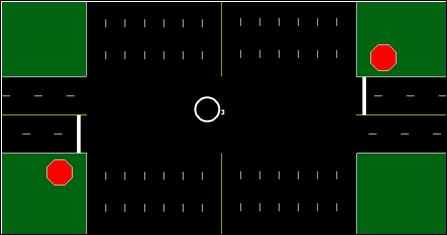
Figure 14 . Illustration. Typical surface street node location.

Surface streets that have opposing overlapped turn bays are offset from the node location so that the node is not at the extension of the left curb, but where the turn bays are overlapped. Figure 15 shows an example of the street placement in TRAFVU when opposing turn bays overlap.

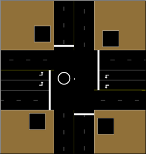
Figure 15 . Illustration. Overlapped turn bay node location.

At the intersection of two one-way streets, the streets will be positioned so that the node will be located at the intersection of the left edges and not in the middle of the intersection. Figure 16 shows the position of one-way streets around a node.

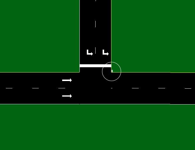
This figure shows the intersection of two one-way streets. The one-way approach from the north intersects the eastbound one-way street in a T intersection. In this type of intersection the links will be placed where the left curbs intersect the node location.

Figure 16 . Illustration. One-way street node location.

Freeway Node Location

Freeway links are positioned so that nodes are located along the left curb of the roadway. This was done for consistency with the arterial streets and so that opposing freeways that are in close proximity can be easily positioned. Two nodes can be located at the same X and Y location to model no median between opposing freeways. Figure 17 shows the freeway placement in TRAFVU for:

Northbound freeway with a right off-ramp fed by a multi-destination lane (a lane where vehicles can either travel straight or exit).
Northbound freeway with a right off-ramp fed by a deceleration lane.
Northbound freeway with a right on-ramp.
Northbound freeway with a left off-ramp fed by a multi-destination lane.
Northbound freeway with a left off-ramp fed by a deceleration lane.
Northbound freeway with a left on-ramp.

Notice that all freeways are placed with the left edge over the node. Notice that the multi-destination lanes appear to be downstream of the node location. They actually start at the node location and are drawn on top of the freeway lanes.

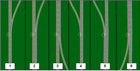
Figure 17 . Illustration. Freeway placement of nodes.

CORSIM can model many types of freeway interchanges but implementing some configurations is not straight-forward. Node placement may require special consideration in these situations. Appendix K shows some ways to model complex link configurations. A freeway node can only have three links connected to it with specific rules on the types of connections and lane alignments.

Interface Node Location

An interface node is a node that connects two different subnetworks (i.e., freeway and surface street subnetworks). When placing interface nodes, select locations that allow the surface street side of the interface to be as long as possible to allow more area for weaving. Vehicles crossing from one type of network to another have very little knowledge of what lies downstream of the interface node. For car-following purposes, vehicles are aware of the next vehicle downstream of the interface node. One of CORSIM’s weaknesses is lane choice of vehicles on multilane interface links. In reality, drivers will often choose which lane to be in while on multilane freeway off-ramps based on their turn decision at the surface street intersection downstream of the off-ramp. The current version of TSIS/CORSIM (version 6.0) has no way to base the freeway off-ramp lane choice based on the downstream surface street intersection turn decisions, which can cause heavy weaving on the surface street of the interface node as turn decisions are assigned after crossing the interface node. This situation can be partially mitigated by placing the interface node as far upstream along the off-ramp as possible to give drivers adequate time and distance on the surface street to react to their upcoming turn.

Layout Nodes in TRAFED

Creating the link-node diagram is accomplished by laying out the nodes in TRAFED. Select either the Surface Node tool or the Freeway Node tool from the TRAFED toolbar and add nodes to the network. Refer to the TRAFED User’s Guide⁽¹¹⁾ for more details on laying out nodes.

An accurately scaled background image can also be used to layout a network. Use caution to be as accurate as possible when scaling the image because even small errors in the scale can lead to large errors in the geometry of the network. The image can also be used as a reference when presenting results. Figure 18 shows the same node layout with and without a scaled background image. It is clear that the background image is useful for orientation of the nodes to the network.

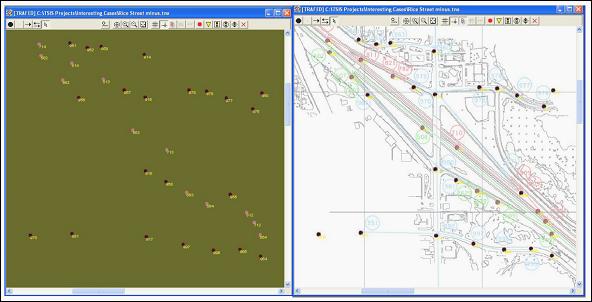
This figure shows a comparison between entering nodes in TRAFED without using a drawing and with a background image to use as an overlay. Using a background image makes it quite clear where the roadways are.

Figure 18 . Illustration. Node layout in TRAFED.

Node Numbering Schemes

The purpose of creating a node numbering convention is to create consistency, which allows for easy review by the model developer and others. By using the numbering sequence presented in this section, sorting links in a sequence that facilitates reviewing and selecting MOEs is an easier process. For instance, if you want to review southbound freeway mainline links, the file can be scanned for nodes that are numbered in the 2000s. Also, combining models becomes an easier process when the likelihood of duplicate node numbers is eliminated.⁽²⁾

Use different sets of numbers to represent different areas of the network. For example, use 1000s for a freeway and 2000s for the opposing freeway. Evens and odds could represent eastbound and westbound or northbound and southbound links. Table 8 shows a recommended scheme for assigning node numbers. The 7000 series of numbers must be used for interface nodes and the 8000 series of numbers must be used for entry nodes.

Table 8 . Sample node numbering scheme.

Node Numbers	Description
1-999	Miscellaneous
1000-1199	Northbound Freeway Mainline
1200-1299	Northbound Freeway Ramps
2000-2199	Southbound Freeway Mainline
2200-2299	Southbound Freeway Ramps
3000-3199	Eastbound Freeway Mainline
3200-3299	Eastbound Freeway Ramps
4000-4199	Westbound Freeway Mainline
4200-4299	Westbound Freeway Ramps
5000-5999	East-West Arterials
6000-6999	North-South Arterials

When assigning node numbers, the node value at the beginning of the roadway should be a low value and increased sequentially as you move down the freeway. Invariably the user will need to add an additional node that will not fit the numbering scheme or require renumbering all the nodes. If gaps are left in the node numbers it is easier to insert nodes into existing links. For example, when numbering the nodes, use 5, 10, 15, 20, and so on. Later a node can be inserted and labeled as number 6 or 7 without having to renumber the whole sequence.

When assigning node values at entrance ramps, it is useful to “pair” the numbers. For instance, if there is a ramp junction node of 110, the first node on the ramp link should be 210. By “pairing” the last two digits of the ramp junction node and the first node on the ramp, you will have another mechanism for reviewing the input file. Depending on the number of nodes on the ramp link, the pairing sequence may not work. The purpose of this pairing concept is to make modeling easier, so be prepared to move onto the next steps if this becomes too complicated. The model will run with any number used as long as it has not been duplicated (with the exception that interface nodes must be in the 7000s and entry nodes must be in the 8000s).

3.2.2 Links

Links in CORSIM are connected to one node on the upstream end and one node on the downstream end of the link. When connecting links between nodes, TRAFED makes the link of the same type as the nodes it is connecting to. When connecting nodes of different types, TRAFED automatically makes a set of interface links and inserts an interface node. If using freehand layout of links, where no nodes exist but are created when the links are created, the default type of link must be set first.

User Link Preferences

Setting the link preferences in TRAFED prior to laying out links may save time later by reducing the changes required for each link. The number of lane preferences for different types of links can be changed to a new number prior to laying out a new section of roadways with similar numbers of lanes. The free-flow speed preference can also be changed to a new speed prior to laying out a new section of streets with similar speeds.

Layout Links in TRAFED

Choose the One-way Link or the Two-way Link tool in TRAFED. TRAFED determines the type of link based on the node it is connecting to. If the user is creating links and nodes at the same time by dragging out the links where no nodes exist, the Default link type will be used. If freeway links are being created with the two-way link tool, only one link will be created because freeway nodes do not service both directions of travel. Click on the upstream node first. In the case of a two-way surface link, it does not matter which node is clicked on first. Move the mouse cursor to the downstream node and click on the node to create the link. If the node is not in view, move the cursor off the side of the view where the node is located. The view will automatically scroll in the direction. The length and direction are displayed in the status bar.

Entry and Exit link descriptions: Entry and Exit links are points where vehicles enter or exit the network. Entry links gather data that can be used for calculating delay. There are no statistics generated for Exit links. To ensure entering vehicles are distributed across all lanes of traffic on the first internal link, make sure the number of lanes on an entry link matches the number of lanes on the downstream link.

The only way in TRAFED to make an entry node and entry link is to drag a link from “greenspace” (where no other object exists) to an existing internal node. The only way to make an exit node and exit link is to drag a link from an existing internal node to “greenspace”. The links and nodes are then created automatically.

Edit Link Properties in TRAFED

Double click on each link or right click and select “Properties” from the popup menu to change the properties of the link. A brief description of some of the link properties for each link and those that are specific to a type of subnetwork is presented in the following paragraphs.

Some link properties that can be set for the link are:

Free-flow speed –the desired, unimpeded mean free-flow speed. It is not the observed speed.
Optional link geometric data
- Lane widths may be input but they are not used to influence driver behavior. They are only used by CORSIM to determine the size of an intersection and by TRAFVU to draw the lanes.
- Link Names – Each link may have a name assigned to it. These names are for reference only. TRAFVU can display these names in different styles, which helps orient an observer.
Graphics – CORSIM was originally designed without concern for graphics. Some parameters have been added to produce graphics. They have no effect on CORSIM operations. Roadway curvature or underpasses/overpasses have no effect on driver behavior or vehicle performance.
- Curve data – affects the display of the link only. The graphic curve data should not be confused with the freeway radius of curvature data that is used to limit the free-flow speed.

Freeway Link Data

Freeway Link Length: In the freeway subnetwork there are no intersections created at the ends of the link; therefore, the link length is also the node-to-node distance (along the curve of the link if curved). However, there may be problems with short freeway links in that vehicles in CORSIM are not allowed to jump over links. Therefore, links should not be any shorter than the distance the fastest vehicle can travel in one time step. On the other extreme, the maximum freeway link length is 30,480 m (99,999 ft) or almost 30.48 km (19 mi).

There are a number of rules for connecting freeway links in CORSIM. Please refer to the CORSIM Reference Manual⁽¹⁾ for more details on the following information.

The maximum number of freeway links at a freeway node is three (two mainline and one ramp link). It is not possible to connect two ramp links and one mainline link. A ramp link cannot be split into two ramp links nor can two ramp links be merged into one ramp. (Appendix K has a discussion of ways to work around this.) Ramp links can connect to only one other ramp, mainline link, or interface link. Mainline freeway links can only have one off ramp at a node (i.e., left and right exits cannot both be located at the same node).

It is recommended that the mainline links be laid out first and then the ramps. TRAFED will automatically make a link a mainline if no other connection at a freeway node exists. If the ramp link is created prior to the second mainline, TRAFED will automatically assign the link as a mainline link. When the second mainline link is added, TRAFED will assign the link as a ramp link. This can get confusing if care is not taken when laying out the links.

Lanes: There are different types of lanes and rules for using them and numbering them. Unlike the surface streets of CORSIM, the freeways must have an equal number of lanes leaving a node as entering. A multi-destination lane leading to an off-ramp is the one and only exception to this rule (see configuration 1 in Figure 17). Use auxiliary lanes and add/drop lanes as a way to ensure the lanes are consistent. Figure 19 shows the freeway lane identification codes. Lanes can be set for different usage including truck bias, truck restriction, exclusive truck lanes, and high occupancy vehicle (HOV) lane operations. Refer to the CORSIM Reference Manual⁽¹⁾ for more information.

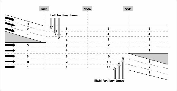
This image is a diagram of the freeway lane numbering used in CORSIM. The five mainline lanes enter from the left and exit to the right. The lanes are numbered 1 through 5, starting at the right. Three on-ramp lanes enter from the upper left and depart to the lower right. The right auxiliary lanes are numbered 9, 10, and 11. The left auxiliary lanes are numbered 6, 7, and 8.

Figure 19 . Illustration. Freeway lane identification codes.

Acceleration/Deceleration Lanes: Acceleration lanes extend from the upstream end of a freeway link to a user-specified mid-link position and must be fed by an on-ramp. Vehicles will use this lane to transition from the on-ramp and merge with traffic on the mainline lanes. Deceleration lanes extend from a user-specified mid-link position to the downstream end of the link and must feed an off-ramp. Vehicles will use this lane to transition from the mainline lanes to the off-ramp. It is possible to have two different auxiliary lanes with the same identification number on the same link. For example, if there are both an acceleration lane and a deceleration lane on the right side, both lanes would be numbered as lane 9.

Full Auxiliary Lanes: CORSIM can have up to three full auxiliary lanes on both sides of the link. A full auxiliary lane extends the entire length of the link. It can connect to a ramp link or it can connect to a mainline lane. Full auxiliary lanes function with the same driver behavior as through lanes. Using full auxiliary lanes, it is possible to model up to 11 lanes of traffic. Figure 20 depicts mainline links with through lanes and full auxiliary lanes that combine to total 11 lanes of traffic. Notice that entry and exit links can only connect to links with, at most, five through lanes. Therefore, to create a segment with more than five lanes, the extra auxiliary lanes must be added and removed at different points along the segment until the desired number of lanes is achieved.

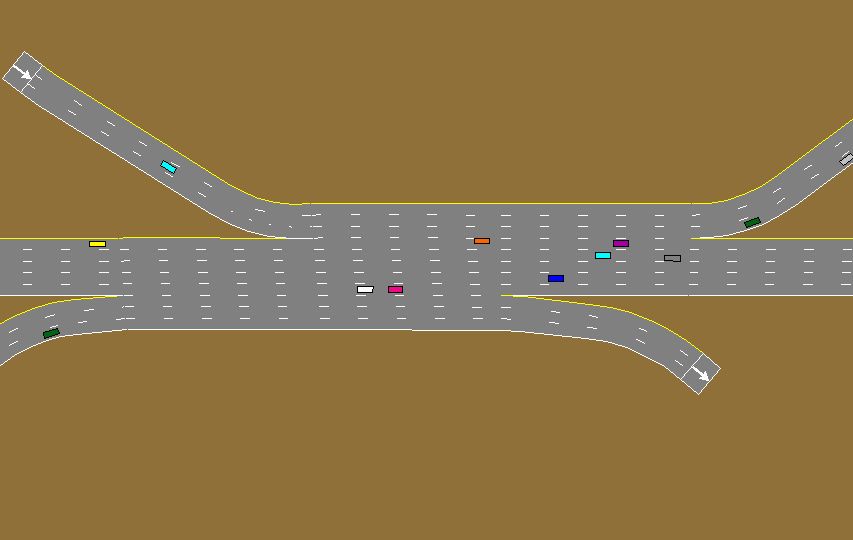
This figure shows a TRAFVU screen of a section of freeway with 11 lanes across. Recent changes to CORSIM allow all left and right auxiliary lanes in the same section.

Figure 20 . Illustration. Freeway layout with 11 lanes.

Add/drop Lanes: Through lanes can be added or dropped at user specified mid-link locations on the mainline or the ramp links. Up to three lanes can be added or dropped on each link. However, the user cannot add lanes to create more than five through lanes on the mainline or more than three lanes on the ramp. The user cannot drop lanes to create a link with no through lanes.

Superelevation, Pavement Friction, and Radius of Curvature

CORSIM provides inputs for superelevation, pavement friction, and radius of curvature that reduce the free-flow speed on the link. CORSIM uses the lower value of the input free-flow speed or the speed based on the calculation from superelevation, friction, and radius of curvature. A warning message is produced if the free-flow speed is set by these inputs. Error checking and calibration may be affected by these inputs if they result in undesirable free-flow speeds. The freeway radius of curvature only affects the free-flow speed; it is not used by TRAFVU to draw links. TRAFVU draws links based on the node locations, link length, and type of curvature.

Barriers

Barriers can be added to prevent vehicles from merging with other vehicles. Barriers can be used to prevent or control a weave zone. Exclusive HOV lanes may be used in conjunction with barriers to model barrier protected HOV lanes. Barriers can also be used to model high occupancy toll (HOT) lanes or HOV lanes that have limited access to the general purpose lanes by placing barriers on the links where access is restricted and no barriers on the links with open access to the HOV or HOT lanes. Barriers do not influence the driver reaction; vehicles will not slow down when next to a barrier nor will they move away from a barrier.

Reaction Points

Vehicles or drivers begin to react to certain roadway geometries and guide signing objects at certain locations. These locations are not necessarily where the traffic sign or feature is located in the real world. (These are also referred to in CORSIM as a “Warning Sign.” This is a poor term that tends to confuse new users into placing them at the location where the actual sign is in the real-world.) The placement of these points is very important to being able to realistically model the real world. In general, drivers do not react to guide signs, but field verification is usually needed to understand how drivers are reacting.

When CORSIM vehicles cross this “reaction point” their lane codes are set so vehicles will begin to move into certain lanes or out of certain lanes. These reaction points have defaultvalues in CORSIM. Measuring this in thefield is difficult, but it can be important to the operation of the network. In the real-world, vehicles that want to exit at a distant off-ramp may not get over until they have passed the location of an intermediate on-ramp. They may move over well upstream because they know the queue builds up well upstream of the off ramp.

Exit-ramps Reaction Point: An off-ramp reaction point should be placed far enough upstream that vehicles in the farthest lane have enough time and distance to move over to position themselves for exit at the off-ramp. The default value of 762 m (2,500 ft) may not be long enough for links with more than two lanes. For example, vehicles in the fifth lane need more space to change lanes prior to reaching the off-ramp. (As a rule of thumb; use 762 m (2,500 ft) plus 305 m (1,000 ft) for each lane greater than two lanes. Thus, five lanes of traffic need about a mile of reaction distance.)

In the case where there are only a few lanes but there is an on-ramp located between the default reaction point and the off-ramp with a large volume of traffic, the warning sign may need to be placed downstream of the on-ramp to model vehicle staying in the left lane until they are past the on-ramp traffic. This congestion due to traffic from the on-ramp is normally handled by Anticipatory Lane Changing (discussed below); however a vehicle that has moved into an appropriate lane for the upcoming off-ramp will not move out of that lane based on the anticipatory lane change logic. Be cognizant of reaction point locations and whether their region overlaps other traffic areas.

Lane Drops Reaction Point: A lane drop reaction point should be placed far enough upstream that vehicles have enough time and distance to move over to position themselves to avoid being stuck at the lane drop location. The lane drop reaction location may need to be moved close to the actual lane drop to allow vehicles to use the lane up to the point of the warning sign. Figure 21 shows the lane drop reaction point downstream of the ramp meter. If the reaction point is upstream of the ramp meter vehicles will avoid using the lane that is dropping.

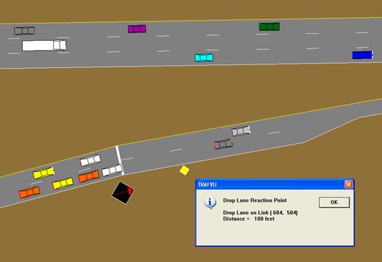
Figure 21 . Illustration. Lane drop downstream of ramp meter.

Anticipatory Lane Change (merge locations): Congestion caused by vehicles entering the freeway from an acceleration lane on a link can cause upstream vehicles to make lane changes away from the side of the freeway where the acceleration lane is located. CORSIM models this behavior with Anticipatory Lane Changing, of which a brief description is given below.

Speed Trigger: The average speed of all the vehicles that are currently on the subject link in the anticipatory region (lanes 1, 9, 10, and 11 for a right-side on-ramp) is evaluated every second. When this average falls below the threshold specified by this entry, anticipatory lane changing will begin. The speed trigger defaults to 2/3 of the free-flow speed. Lane changing will only happen if there is no disadvantage in the lanes of the non-anticipatory region. If the average speed increases to a value above the threshold, anticipatory lane changing will cease in this region.

To prevent anticipatory lane changing in this region, enter a very low minimum speed, such as 1.6 km/h (one mi/h). To maximize anticipatory lane changing in this region, enter a very high minimum speed, such as 159.3 km/h (99 mi/h).

Distance to React: Congestion caused by vehicles entering the freeway from an acceleration lane on this link can cause upstream vehicles to make lane changes away from the side of the freeway where the acceleration lane is located. The distance upstream to the point at which vehicles will react to the congestion is determined by this entry, measured in feet from the upstream end of the link. If the speed threshold has been exceeded, the desire to perform the lane change will increase linearly from the minimum value to the maximum value as the vehicle travels between the upstream reaction point and the upstream end of the subject link.

Anticipatory lane changing can be prevented by specifying a very short reaction distance, such as one ft. To simulate a recurring congestion problem caused by an on-ramp, use a long distance to model vehicle moving over in anticipation of the congestion that is present on a daily basis.

HOV Lane Reaction Point: This is the location where HOV vehicles begin to react to an upcoming HOV lane. HOV vehicles will begin to change lanes in order to position themselves for entry into the HOV lane.

HOV Exit Reaction Point: This reaction point defines the upstream location for an HOV exit warning sign. All HOV vehicles that will be exiting the freeway from this link will avoid exclusive HOV lanes after passing this warning sign. If they are currently in an exclusive HOV lane they will attempt to exit from that HOV lane as soon as possible. This entry has no effect on other vehicles and only affects HOV vehicles when exclusive HOV lanes have been entered. This value must be greater than or equal to the off-ramp reaction point.

3.2.3 Surface Street Link Data

There are a number of considerations specific to surface street link data including link length and lane data.

Link Length

Link length is measured from the stop bar of the upstream link to the stop bar at the downstream node including the upstream intersection if there is one. TRAFED uses the node-to-node distance when assigning the original link length. If the user has not changed the link length from the node-to-node distance, dragging the node at either end automatically changes the link length. Once the link length has been changed by the user and is no longer equal to the node-to-node distance, dragging a node will not change the length of the link.

In some cases, the link length will correspond to the node-to-node distance. In other cases, the two measurements can be significantly different. For example, consider two parallel but opposing streets with no intersection at one end and a seven-lane intersection at the other end. Figure 22 shows that two such parallel links can have significantly different link lengths. The links were both unchanged from the length that TRAFED created them, 500 ft. The westbound link should be 584 ft from stop bar to stop bar. It shows vehicles in a queue spaced widely apart. The eastbound link should be 416 ft from stop bar to stop bar. It shows vehicles overlapped due to the discrepancy between the input length and the actual length.

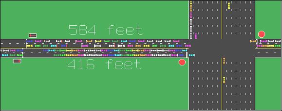
Figure 22 . Illustration. Effects of incorrect link length.

If the length is not correct, CORSIM may be able to store more or less vehicles on the link than can be stored in the real world. CORSIM may allow more vehicles on a link than is possible in the real world because the link length was not accurate, or CORSIM may not allow as many vehicles on the link as the real world link can hold.

TRAFVU animation will show problems with the link length in different ways. Overlapped vehicles will show up when the link length, as determined by TRAFVU, is less than was input to CORSIM. (i.e., CORSIM calculates that there is more storage than there actually is.) Also, vehicles will appear to animate very slowly across these links. Use the TRAFVU Link Properties to show the input length and the TRAFVU calculated length for comparison. If the input length is shorter than TRAFVU determines is required based on the geometry, vehicles will be spaced very far apart when in queue. (i.e., CORSIM calculates that there is less storage than there actually is.) Vehicles will also animate very fast across these links.

Lane Data

Links are the main connector from node-to-node, but it is at the lane where vehicles interact. Lanes can vary in width from lane to lane and from link to link, however, lane width does not affect driver behavior in CORSIM. The only use for lane width in CORSIM is to determine the size of an intersection. Lane width is used by TRAFVU to draw links, lanes, and intersections.

CORSIM does not have the capability of modeling partial lanes or placing vehicles in two lanes at the same time. Vehicles always travel in a specific lane. Any animation effect that shows vehicle crossing the lane line during lane changing is done by TRAFVU as it interpolates the vehicles position from one second to the next. This becomes significant when modeling tapered lanes and modeling links that merge with other links at shallow angles.

TRAFVU Surface Street Intersection Pull Back Description: The way an intersection is created and drawn in TRAFVU is to lay down the end of the left curb of all the links at the node and then pull them back to the point that they do not overlap. This works fine for perpendicular roadways, but links that approach a node at shallow angles tend to pull back a long way. This also shortens the adjacent links considerably. With very little graphical information, there is no other way to do this. There is no drop lane or acceleration lane concept on the surface street. One method to work around this situation is by connecting to a full lane that drops at the next node. The top drawing in Figure 23 shows how TRAFVU draws the links when they merge at shallow angles and the bottom drawing in the figure shows the work around to the link pull back problem. This method requires adding a short link with an extra lane of traffic that the vehicles use to merge with the through lanes.

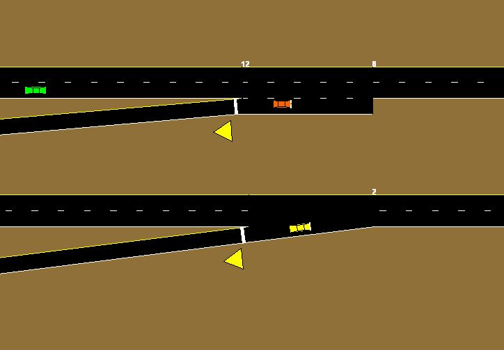
Figure 23 . Illustration. TRAFVU intersection pull back.

Lane Numbering Diagrams: There can be up to seven lanes on each surface street. There can be two turn bays on each side of the street. If there are two turn bays on each side of the street, there can only be three through lanes. Figure 24 shows the lane numbering scheme for surface streets. It is important to understand how CORSIM numbers the surface street lanes for placement of detectors and for assigning channelization.

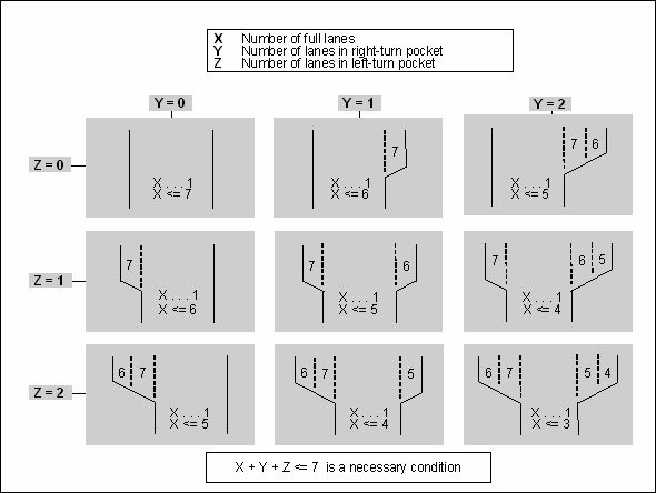
This figure is the surface street lane numbering scheme used by CORSIM. The left and right turn lanes are numbered starting at seven and working backwards. The main lanes are numbered starting at one and increasing. The total number of lanes cannot exceed seven.

Figure 24 . Chart. Surface street lane numbering.

Lane Channelization: Lanes can be channelized for different types of traffic flow (turns) or for special utilization. Unfortunately, turn movements and utilization cannot be combined. Surface street lanes in CORSIM can have special utilization including buses only, carpools only, or closure. Lanes can alternately be channelized for left, right, through, or diagonal movements, or combinations of these movements. Turn bays are automatically channelized to the corresponding turn movement. They do not need to be set nor can they be changed. Turn bays that are the full length of the link should be coded as channelized full lanes because upstream feeder links cannot connect to a full length turn bay. Figure 25 shows full left turn lanes channelized for left turns only.

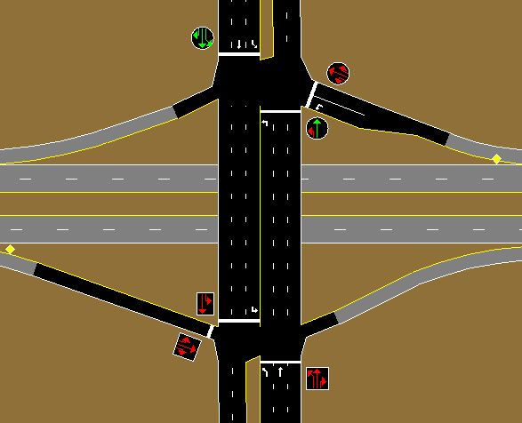
This figure depicts a typical diamond intersection as drawn in TRAFVU. The left turn lanes are full lanes that are channelized for left turn only. If left turn bays are used they cannot extend the full length of the link. Vehicles approaching from upstream will not be able to enter a full length turn bay because it does not connect at the intersection. A full lane must be used in this situation.

Figure 25 . Illustration. Left turn channelization.

Lane Alignments versus Turning Alignments: The lane alignment and turning alignments are sometimes confusing. Lane alignment is for through movement. CORSIM and TRAFVU use lane alignment to align the intersection. By default, lane 1 on the upstream link aligns with lane 1 on the downstream link. However, lane 1 on the upstream link may align with lane 2 on the downstream link or lane 2 on the upstream link may align with lane 1 on the downstream link. Figure 26 shows both lane alignment situations.

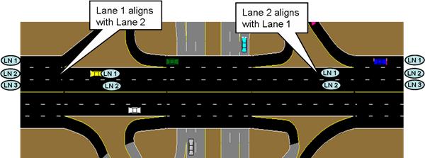
Figure 26 . Illustration. Sample lane alignment.

On the other hand, the turning alignments are used to restrict vehicles to turn into certain lanes or allow them to turn into additional lanes. By default, CORSIM only allows vehicles to turn from the near lane on the upstream link to the near lane on the downstream link. Turning alignments do not need to be set unless vehicles should be allowed to turn into other lanes. Figure 27 shows such a situation.

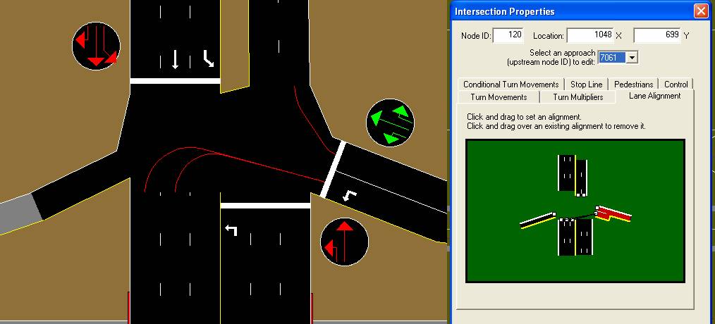
Figure 27 . Illustration. Turning alignments.

A unique lane channelization, lane alignment, or turning alignment may be needed in the base CORSIM model to replicate an existing condition. The analyst should take note of these unique features and be sure to revisit them in the alternatives analysis step, as a unique geometric feature in the existing conditions may be fixed or altered in a future case alternative.

3.2.4 Corridors

Surface street subnetworks and freeway subnetworks can be connected to form a corridor where the two subnetworks interact. Interface nodes are used to connect the two subnetworks. Only two links can connect at an interface node. TRAFED will connect the two subnetworks and add the necessary interface nodes by simply dragging a link between the two different subnetwork nodes. The number of lanes must match on both sides of the interface node. Mainline freeway links and ramp links can connect to surface links directly at the interface node.

3.2.5 Review

At this point in the base network development, the network will not run in CORSIM without more modifications, but it can be viewed in TRAFVU. This is a good checkpoint. Save the TRAFED network and save it (translate it) to a TRF file. Then open the TRF file with TRAFVU and review the geometry of the network. This is a cursory review of the network; a detailed review and error checking will come later. For large networks, performing a cursory review of the link-node diagram at multiple points of development (e.g., after the freeway is coded or after each interchange is coded), rather than only at the conclusion of the network, would help ensure errors are caught early in the coding process

3.3 Traffic Demand Data

The demand data consists of Entry Volumes, Turn Volumes or Turn Percentages, Origin-Destination data, and Vehicle Mix.

3.3.1 Entry Volume

Entry points describe the volume, in either vehicles per hour or traffic counts for the time period, entering the CORSIM network. Counts will be changed into hourly equivalents within CORSIM so that entry headways can be easily calculated.
Entry volumes are required for all freeway networks and surface street networks that do not use the traffic assignment option. The traffic assignment option used to generate surface street traffic volumes does not require entry volumes entered at entry points. Using that option requires entering the volume of traffic in the origin-destination trip table (see “Surface Street Demand” discussion in this section for more detail).

Entry nodes usually form the outer boundary of the network. The network will normally receive traffic from entry nodes on its periphery. The exception to this is large internal traffic generators or receivers such as parking garages, side streets, or neighborhoods that can be modeled as internal entry nodes with their own traffic volumes.

Entry links are unique in that they are not part of the network itself. As vehicles are generated by CORSIM, they are accumulated on the entry links for later discharge onto the network from the entry link. The car-following, control, and spillback conditions at the downstream node of the entry link regulate entry of vehicles onto the network. Network statistics are not accumulated for the entering vehicles until they have left the entry link. The entry volume must also specify the percentage of vehicles of each type. Carpool and truck percentages must be defined explicitly. By default, no carpools or trucks are part of the traffic flow. When carpool and truck percentages are input, the car percentages are defined by subtracting carpool and truck percentages from 100 percent. Bus volumes are not part of the entry volume and are defined separately.

Specified entry point volumes cover all lanes of the link; they are not specified on a per lane basis. The maximum number that can be entered for an entry point is 9,999 vehicles for a given time period. Thus for a one hourtime period, this equates to slightly less than 2,000 vehicles per lane for a five-lane freeway or slightly more than 1,400 vehicles per lane for a seven-lane surface street. If higher volumes are required, they can be entered as counts with time period durations less than one hour or using volumes that vary within a time period. Refer to volume variations within a time period in the CORSIM Reference Manual⁽¹⁾ for more information.

Time Period Varying Demand

CORSIM can capture the onset, presence, and dissipation of congestion by varying the input volume over multiple time periods. Specified entry link volumes will stay in effect until the end of the simulation unless changed bysubsequent entries in the same period or in later periods. The volume will be smoothly increased or decreased to adjust to the new volume input in a different time period. If a subsequent time period has no changes and then a later period includes inputs that specify different entry volume, the volume through the period for which no entry volumes were specified will be linearly interpolated between the specified volume at the end of the previous period and the specified volume at the beginning of the next period.

For example, if a simulation includes three time periods where an entry volume of 1,000 vehicles per hour was specified for time period one, and no subsequent time period includes any changes to the volume, the volume will remain constant at 1,000 vehicles per hour for all three periods. However, if there is an entry for time period three that changes the volume to 2,000 vehicles per hour, but no change was entered for time period two, then the entry link volume will vary throughout time period two, starting at 1,000 vehicles per hour and increasing to 2,000 vehicles per hour at the end of the period. Figure 28 shows a graph of this example. The lower line depicts explicitly setting the volume during the second time period to 1,000 vehicles per hour.

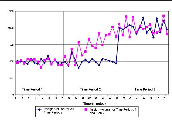
Figure 28 . Graph. Volume interpolation when not assigned for a time period.

When entry link volumes are not constant throughout the simulation, the best way to be sure that the volumes are correct is to specify the volumes explicitly for each time period.

Sub-time period varying demand: The analyst can specify variations in entry volumes within a time period. The analyst can specify up to 16 variations in volume for each time period. If the entries are specified in vehicles per hour, CORSIM will interpolate between the data points to determine flow rates at times between the specified times. If the entries are specified in vehicle counts, CORSIM will calculate the required flow rate to generate that number of vehicles over the specified time interval.

Some valid uses of sub-time period variations are:

More variations in the volume are necessary (CORSIM only allows 19 time periods).
The volumes change more frequently than on the time period boundary. For example, each time period is defined as 15 minutes long but the volume data are in five-minute intervals.
There is no need for time period reporting or other variations that would require the use of time periods. All input volume can be done through sub-time period entries.

Vehicle Entry Headway

Vehicle entry headway is the time between one vehicle entering the network and the previous vehicle to enter the network. The headway is defined as 3600 divided by N, where N is the hourly volume in vehicles/hour. CORSIM can generate these headways deterministically, using a constant headway (which is the default), or stochastically using either a normal or an Erlang distribution. The type of headway applies to the whole network and cannot be modified for individual links (i.e., a global parameter). See appendix E for more details. The three types of headways are briefly described below:

Constant Headway: All vehicle entry headways are set equal to the constant headway, defined as 3600 divided by N, where N is the hourly volume in vehicles/hour. This produces a constant stream of vehicles. Use constant headway to model an upstream stop sign or ramp meter flow metering. It is also useful when performing traffic modeling research where no variation in the vehicle injections is desired.
Normal Distribution: This distribution produces a truncated bell curve of entry headways. The headway, defined as 3600 divided by N, where N is the hourly volume in vehicles/hour, is used as the mean value for the distribution. If headway values less than the minimum value are produced, a redraw of the value is performed. This distribution produces platoons of vehicles instead of a constant flow.
Erlang Distribution: This produces different distributions of entry headways determined by the Erlang parameter. The distributions can vary from an exponential distribution to a normal distribution. The headway, defined as 3600 divided by N, where N is the hourly volume in vehicles/hour, is used as the mean value for the distribution. If headway values less than the minimum value are produced, a redraw of the value is performed. This distribution provides more variation in vehicle headways than constant or normal distribution. See appendix E for detailed discussion and graphs of the Erlang distribution.

While the default setting is a constant headway, a stochastic distribution (Normal or Erlang) would be more appropriate for real-world applications to account for natural randomness in driver behavior. In the absence of field measured headways, an Erlang Distribution with a =1 may be used, which replicates a negative exponential distribution. A negative exponential distribution is commonly used for generating the inter-arrival time of “customers” (e.g., vehicles) to a system. Refer to appendix E for more information on headway distributions.

3.3.2 Freeway Demand

The freeway subnetwork has some specific considerations related to demand inputs including origin-destination data, off-ramp turning percentages, minimum separation of entering vehicles, and the distribution of vehicles between lanes.

To code the freeway traffic volume data, entry volumes and turning percentages are required, while origin-destination (O-D) data is optional. There are three approaches to entering freeway demand data: 1) entry volume data and turn percentages; 2) entry volume data, turning percentages, and complete O-D data, or 3) entry volumes, turning percentages, and partial O-D data. The most straightforward way to enter freeway demand data is by using entry volumes and turn percentages (approach 1).

Approach 1: Complete Turning Counts or Percentages

In this approach, the counts of vehicles or percent of traffic should be specified for every node that has an off-ramp. If turn specifications are entered in the form of vehicles/hour, CORSIM will internally convert these inputs to turn percentages. Entry volumes are used to generate the actual number of vehicles on the network, whereas turning counts are used strictly to assign relative turning movements of these vehicles that entered the network.

The freeway entry volumes and turning percentages at ramp exits are internally converted to an O-D table. The gravity model is designed to perform this conversion. More information about the gravity model as applied in CORSIM can be found in the CORSIM User’s Guide.⁽¹⁾

Vehicle Type-specific Turn Movements: By default, the turn percentages at an off-ramp apply equally to all vehicle types. It is possible to specify that certain vehicle types have different turning fractions for specific off-ramps. If altering the turning percentages for a specific set of vehicle types, it may be necessary to set all vehicle types to ensure the overall exiting volume remains correct. An example of when this is useful is when modeling the effects of a truck weigh station. A high percentage of the trucks would be assigned to the exit and a very low percentage of other vehicle types would be assigned to the exit. This vehicle type-specific turn movement is not necessary for buses and will not have an effect on buses.

Approach 2: Complete Origin-Destination Data

The number of vehicles that exit at an off-ramp can also be specified through O-D data. The trip table from the origin to the destination specifies the percentage of traffic that will exit at individual destinations from an origin node. The destination volumes are modeled by linear systems according to the input data. An iterative process is used to solve the linear systems. Where there are groups of freeway interchanges, in some rare cases, the sufficient condition for the convergence of the linear systems cannot be satisfied. Consequently, the destination volumes may not converge. If that happens, a warning message will be generated by CORISM.

Even when the complete O-D data set is known, the analyst must still specify entry volumes and exit percentages. CORSIM will use that data to create an internal table of origin volumes versus destination volumes. O-D data can be used to ensure that the correct origin-destination relationships are enforced, but CORSIM will attempt to balance all of the information from the three input types. Therefore, it is important that the entry volumes and turn percentages are consistent with the O-D data. The analyst may find it useful to develop a spreadsheet to estimate entry volumes and exit percentages based on the known O-D data.

The analyst is responsible for ensuring that the traffic volumes for all destination nodes agree with the traffic volumes entered using input data. Otherwise, the origin-destination table may not be balanced. If that happens, a warning message will indicate the unbalanced volumes at specific exit nodes. The analyst should make the necessary change. If the convergence could not be achieved and/or the O-D table could not be balanced, CORSIM can still run. However, CORSIM can not assign the correct volumes on all links. CORSIM will report the O-D tables to assist the analyst in debugging the O-D input data. The analyst can increase the number of iterations to improve the convergence.

Approach 3: Partial Origin-Destination Data

If entry volume and turn percentage data are available, but at the same time it is important to maintain some of the O-D pairs, CORSIM will first calculate destination volumes based on a linear system equation model by entry volume and turn percentage. Second, CORSIM utilizes the input O-D data to “override” CORSIM calculated O-D pairs. CORSIM then calibrates the O-D pairs without the specified input O-D data. Finally, a balanced O-D table is generated. However, the “override” makes sense only when the O-D table can be balanced. In this case, it is suggested that users prepare entry volumes, turn percentages, and O-D data, then perform a CORSIM run and check for warning messages. If warning messages are generated, follow instructions in the CORSIM Reference Manual⁽¹⁾ for O-D data to try to eliminate the warning message. For a simple FRESIM network, you may want to generate a complete O-D pair table first, then, follow the steps outlined in the previous situation. For a complicated network, you can check the CORSIM O-D table output and make necessary changes to the turn percentages and/or O-D data.

Using partial freeway O-D trip data, it is possible to control traffic flow on an individual interchange basis. In CORSIM, the percentage of vehicles exiting at the off-ramp does not depend on where the vehicle entered the freeway unless O-D is used. In most real world situations, traffic entering the freeway at an on-ramp probably does not exit at the next off-ramp. Modeling this weave zone correctly can improve the comparison to the real world. Using O-D trip tables helps prevent vehicles from continuously traveling on a clover-leaf. Figure 29 shows a situation where very little traffic would enter the freeway at point A and then immediately exit at point B. Using the O-D trip table, the percentage of traffic that has an origin of A and a destination of B could be set to zero.

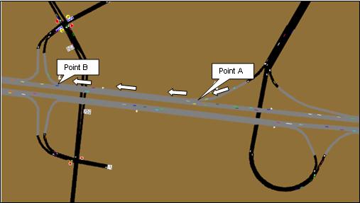
Figure 29 . Illustration. Ramp-to-ramp trips.

Minimum Separation of Vehicle Generation

The minimum separation for generation of vehicles governs the maximum rate at which vehicles on a single lane freeway can be emitted onto the network in a given lane. Overall, the rate that vehicles are emitted is governed by the volume of traffic entering the network at a certain location. If the input volume is greater than 2,250 vehicles per hour per lane, the default minimum separation of 1.6 seconds will not allow all the vehicles to enter the network. To achieve 2,400 vehicles per hour per lane, the minimum separation must be reduced to 1.5 seconds (i.e., 3600/1.5 = 2400). This is a network-wide parameter that affects all freeway entry points, and it should be adjusted to accommodate the highest entry volume in the network.

Distribution Among Lanes

The distribution of vehicles entering different freeway lanes can be defined by the user to model real world distributions. For example, across three lanes of traffic 50 percent could be assigned to lane one and 30 percent to lane two and 20 percent to lane three. This can be used to model the effects of an on-ramp upstream of the entry point where many vehicles are still in the lanes coming from the on-ramp when they reach the entry point. The percentage of vehicles entering each lane is based on the total flow rate specified. The sum of the percentages must equal 100 percent. Downstream of the entry point, vehicles will begin to change lanes for discretionary or mandatory purposes so the lane distribution will not stay in effect downstream of the entry point.

3.3.3 Surface Street Demand

Turn Percentages

Turn movement percentages only apply to passenger cars, carpools, and trucks. Bus turn movement data is based on the specified bus path data. All traffic exiting on interface nodes must travel straight through to the next network. Turn movement data can be entered for each time period to reflect the changes in turn percentages or traffic blockages.

If turn specifications are entered in the form of vehicles/hour, CORSIM will internally convert these inputs to turn percentages. If the entries do not total 100, CORSIM will treat them as volumes and will convert them into percentages. Entry volumes are used to generate the actual number of vehicles on the network, whereas turning counts are used strictly to assign relative turning movements of these vehicles that entered the network.

Vehicle Type-specific Turn Movements: The turn percentages at an intersection apply equally to all vehicle types. It is possible to indicate that certain vehicle types have different turning fractions for specific intersections that have an associated turn.

Interchange origin-destination

Multilevel urban interchanges can be modeled in NETSIM. To assist in the coding of interchanges, there is an option of entering travel demand patterns (i.e., O-D information) through an interchange instead of turn percentages for each link.

Conditional Turn Movements

Conditional turn movements can be used to prevent vehicles from making a series of unrealistic turn movements. For example, at a diamond interchange, the user may want to prohibit vehicles from making a left-turn to an on-ramp when they just made a left-turn from an off-ramp (i.e., restrain vehicles from returning to the freeway when they just exited the freeway). The NETSIM model normally applies the specified turn movement percentages to all vehicles entering a link, regardless of their previous path. CORSIM allows the user to define discharge turn percentages that are conditioned on the basis of entry movement. Therefore, the percentage of vehicles executing left turns after entering via a left turn can be made substantially less than the percentage of vehicles executing left turns after entering via a through movement.

If the user defines turn percentages for one entry movement–exit movement combination, they must define the discharge turn percentages for all other traffic entering the link. When discharge turn percentages are defined for traffic entering from some directions and not from others, the traffic entering from the remaining directions is assigned discharge movements subject to the turn percentages of each turn movement defined. This could result in undesirable turning volume.

For example, Figure 30 shows a typical diamond interchange. The original traffic counts may have shown that 20 percent of the vehicles on the southbound link turn left to the eastbound on-ramp. Without conditional turn movements, on average 20 percent of the vehicles that came from the westbound off-ramp would turn left at the on-ramp (approximately 40 vehicles over an hour). With conditional turn movements, that number can be changed. If zero vehicles that came from the westbound off-ramp should turn left onto the eastbound on-ramp, all 200 vehicles per hour will travel southbound through the intersection. If the number of vehicles that came from the upstream southbound link is not changed by using the conditional turn movement also, only 20 percent (i.e., 200 vehicles) of the 1,000 vehicles per hour will turn left. However, since 1,200 vehicles travel on the link per hour, a total of 240 vehicles (20 percent of 1,200 vehicles) should be making a left turn at the intersection. For an accurate representation of the field data, the analyst must also specify conditional turn movements for the vehicles entering the approach link via a through movement. Conditional turn movements must be specified so that 24 percent of the vehicles entering via the through movement turn left onto the on-ramp while 76

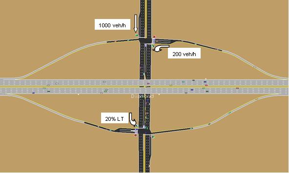
Figure 30 . Illustration. Conditional turn movement example at diamond interchange.

Origin-Destination Trip Table

Specification of the trip table can be entered in the form of origin-and-destination nodes. Sources and/or destinations (sinks) of traffic that are internal to the network can also be specified. When traffic assignment is requested, all record types relating to entry volumes and turn movements should be left out of the dataset; the volumes and percentages will be determined by the traffic assignment results.

Due to the unspecified volume of traffic entering the surface street subnetwork from a freeway subnetwork at an interface node, traffic assignment can only be performed when surface streets are the only links in the network. At the time the traffic assignment model was developed, the interface with a freeway subnetwork was not an option. If traffic assignment must be used, the surface street subnetwork must be developed prior to the freeway subnetwork or the freeway subnetwork must be developed separately and combined after traffic assignment has been run and turning percentages have been calculated.

Another limitation of traffic assignment is that it is not entirely accurate when intersections are controlled with actuated control. This is due to the uncertain amount of green time during a phase. If traffic assignment must be used, the surface street subnetwork must be developed with fixed time control with appropriate green times. After traffic assignment has been run and turning percentages have been calculated and input into the model, the controllers can be changed to be actuated control.

Although traffic assignment models are not categorized as simulation models, they represent an essential interface between travel demand and actual traffic flows. Assignment models convert O-D trip tables into estimates of network loadings, which can then be used by simulation models to evaluate the network performance as well as demand responses to operational changes. The purpose of the traffic assignment feature for surface streets is to generate an estimate of turning volumes, or percentages, at intersections. The analyst should review the assigned turning volumes, or percentages, at specific intersections after performing a CORSIM run with surface street traffic assignment. Adjustments may then be needed to the turning volumes to better match actual traffic flows. Refer to the CORSIM Reference Manual for more information on traffic assignment.

Source-Sinks

Source/sink locations represent net flow for the entire block. They represent the net gains or losses for all parking lots or garages on the links and the net curb parking turnover. Source/sink locations are best for representing places with flow that occurs predominantly in one direction. If there are minor streets such as alleys, business or retail driveways, or stop sign controlled minor streets with only two or three vehicles per hour on the link, they would also be included in this number. Therefore, source/sink locations are pseudo nodes representing the aggregate of many minor traffic activities, and are not real nodes representing a single traffic activity. Entry/exit links can be used within the network for locations that both generate traffic and remove traffic from the network (such as very large parking garages).

Negative flow values are specified for net flow off of the street. Positive flow values are specified for net flow onto the street. For example, ten vehicles per hour enter the street from a bank driveway but fifteen vehicles per hour leave the street into a strip mall 30.5 m (100 ft) downstream. These could be represented with a single source/sink with negative five vehicles per hour flow rate. Thus, source/sink locations can be used to reconcile minor differences between the number of vehicles entering and exiting a link.

CORSIM treats the activity of the source/sink centroid as occurring mid-block. There is no disruption of the traffic flow when an auto or truck enters or exits the link (buses are not affected by source/sinks). Vehicles simply appear or disappear from the street at the location of the source or sink without disrupting traffic (i.e., they do not slow down to exit). If there are major sources or sinks with continuous in and out activity that disrupts traffic flow through the time period, then these should be modeled as side streets with entry nodes and not with source sink locations.

For the purposes of counting trips, vehicles that come from source nodes or that exit at sink nodes only count as half a trip because they only traveled half of the link. Vehicles entering from a source node travel the downstream half and vehicles exiting at a sink node travel the upstream half of the link. When COSRIM reports the number of vehicles discharged it reports all of the vehicles that reach the end of the link and get discharged onto the next link. It does not matter if they entered the link from a source node or if they entered the link from an upstream link.

3.3.4 Vehicle Mix

CORSIM allows four different fleets (passenger car, truck, bus, and carpool) and defaults to nine vehicle types. The vehicle mix is defined by the analyst, often in terms of the percentage of vehicles types at each entry node. Typical vehicle types in the vehicle mix might be passenger cars, single-unit trucks, semi-trailer trucks, and buses. Default percentages are usually included in most microsimulation programs; however, vehicle mix is highly localized and default values will rarely be valid for specific locations. For CORSIM, the default is for passenger cars only. If other vehicle types are required the analyst will need to input these values. A detailed discussion on vehicle mix is provided in appendix A.

3.4 Traffic Control

There are four types of traffic control data in CORSIM: freeway ramp meter data, sign control data, actuated signal control data, and pre-timed signal control data. Each of these control types is discussed in the remainder of this section.

3.4.1 Freeway Ramp Meter Control

CORSIM defines five types of on-ramp signal control strategies and the location of the detectors necessary for the application of metering strategies. The user may also specify an externally-defined ramp meter type that is not implemented inside CORSIM and that must be controlled using a Run-Time Extension (refer to appendix L for more information).

Detectors must be set on the appropriate links for ramp meter controls that use thresholds for adjusting the metering rate. These should be set prior to setting up a traffic responsive ramp meter. The practitioner should be aware that once ramp metering is initiated in a simulation run, it cannot be “turned off.”

Clock-time

To simulate clock-time control of the on-ramp, a single, fixed headway is specified. The meter’s countdown clock is initialized to this value at the beginning of the red indication and the signal is set to green each time the clock expires (returns to zero). For typical project/design analysis, the clock-time metering is usually sufficient control to evaluate project design alternatives.

Demand/Capacity

The demand/capacity metering algorithm performs an evaluation of current excess capacity, immediately downstream of the metered on-ramp, at regular intervals, based on counts from the surveillance detectors on the freeway mainline. A maximum metering rate is calculated such that the capacity of this freeway section is not violated. In addition to the specification of the capacity, the user must specify the detectors on the link that will provide the input to the metering algorithm.

Speed Control

The algorithm for this form of ramp metering is similar to the demand/capacity strategy. A freeway link detector station must be established and identified at which speeds are evaluated and used to establish a metering rate. Generally, this detector location will be upstream of the on-ramp, although the logic does not preclude other placements. The user must specify a table of speeds and metering headways for the on-ramp. As each evaluation period concludes, the prevailing speed at the freeway detector station is compared to the tabulated minimum speeds to determine the proper metering rate.

Multi-threshold Occupancy

The algorithm for this form of ramp metering is similar to the demand/capacity strategy. A freeway link detector station must be established and identified at which occupancies are evaluated and used to establish a metering rate. Generally, this detector location will be upstream of the on-ramp, although the logic does not preclude other placements. The user must specify a table of occupancies and metering headways for the on-ramp. As each evaluation period concludes, the prevailing occupancy at the freeway detector station is compared to the tabulated minimum occupancies to determine the proper metering rate.

ALINEA Control⁽⁹⁾

The ALINEA ramp metering control uses a feedback strategy based on a linear regulator control system. ALINEA is an acronym for the French “Asservissement Linéaire d’Entrée Autoroutière”, which loosely translates to Linear Control of Entries to Motorways. More information on ALINEA metering is available in the TRAFED User’s Guide.⁽¹¹⁾

HOV Bypass Lane

If an HOV lane exists at a ramp meter, the ramp meter will not control the HOV lane. The vehicles in the HOV lane will bypass the ramp meter.

3.4.2 Arterial Control

Sign Control

Stop and yield signs can be modeled in CORSIM. The signs are placed at the downstream end of the approach link. Any or all approaches to an intersection may be stop sign controlled. All-way stops are implemented so that the first vehicle to reach the stop bar will have the right-of-way to discharge first.

Sign control and right turn on red are subject to the gap acceptance parameters set in CORSIM. The gaps for right turning vehicles are checked against vehicles approaching from the left. Gaps for left turning vehicles are checked against vehicles approaching from the left, the right, and from the opposing link. The gap acceptance parameters can have a significant effect on the operation of sign control and should be calibrated to local conditions as necessary (see discussion on calibration in Chapter 5).

Actuated Signal Control

The actuated control model in CORSIM is an implementation of an eight-phase, dual-ring NEMA controller, as specified in the NEMA TS 1 and TS 2 standards. The model can be configured to emulate the operation of a Model 170 controller and many of its features, but the CORSIM terminology is taken from the NEMA specification. Figure 31 shows a sample TRAFED Actuated Control dialog screen. Refer to the TRAFED User’s Guide⁽¹¹⁾ for specific guidance on inputting data. It should be noted that it is possible to create arterial networks with signal control in Synchrotm and transfer the network to CORSIM for analysis. Additional details of this process are described under signal optimization, discussed later in this section.

The CORSIM actuated controller can be configured to operate in one of three modes: fully actuated, semi-actuated, or semi-actuated coordinated. In fully-actuated mode, detection is provided on all approaches to the intersection, and the controller operates without a common background cycle (i.e., operating “free”). In semi-actuated mode, detection is provided only on the side-street approaches (and perhaps main-street, left-turn movements). The main street signals remain green until a call for service is placed by the side-street detectors. In this mode, the controller operates without a common background cycle (i.e., operating “free”).

Semi-actuated, coordinated operation is used to provide progressive vehicle flow through a series of controlled intersections. In this mode, each controller in the coordinated system operates within a common background cycle length. The coordinator in the controller guarantees that the coordinated phases (generally phase 2 in ring 1 and phase 6 in ring 2) will display green at a specific time within the cycle, relative to a system reference point established by the specified cycle length and system synch reference time. An offset time, relative to the system reference point, is specified for each controller in the series to maintain the smooth progression of vehicles through the intersections. The coordinator also controls when and for how long non-coordinated phases can indicate green so that the controller will return to the coordinated phases at the proper time. A detailed discussion of Actuated Control as implemented in CORSIM is documented in appendix F.

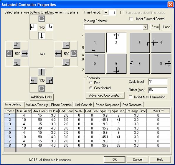
Figure 31. Illustration. TRAFED actuated control property dialog.

Pre-timed Control

Pre-timed signals can also be modeled in CORSIM. The models can simulate a multiple-dial traffic control system in which pre-timed timing plans can vary in offset, interval durations, and signal codes from one timing plan to another. The approaches to the intersection, the number of signal intervals, and the duration of each interval must all be input as well as the control facing each approach during each interval, such as green ball, amber ball, red ball, and green left turn arrow. If a left turn has an opposing through movement, CORSIM internally makes the turn permitted. Figure 32 shows a sample TRAFED Pre-timed Controller Property dialog screen. Refer to the TRAFED User’s Guide⁽¹¹⁾ for specific guidance on inputting data.

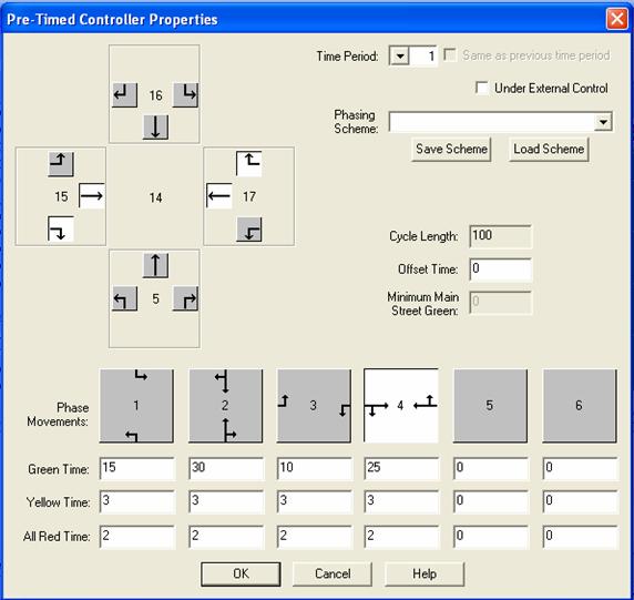
This figure is a TRAFED Pre-Timed Controller Properties dialog box for a typical intersection. The approach movements are shown on the upper left side of the box. The Time Period, and Offset Time are input on the upper right side of the dialog box. The Phase (Interval) Movements are selected along with the Green Time, Yellow Time, and All Red Time are input along the bottom of the dialog box.

Figure 32 . Illustration. TRAFED pre-timed controller property dialog.

Amber intervals for single movements (e.g., left-turn arrows and right-turn arrows), with other movements retaining the green, are computed internally by the models. For these movements, the user specifies an amber code for the approach for the movement specific amber interval. The user then specifies the appropriate code for the green indications in the subsequent interval. CORSIM internally computes to which movement(s) the amber is applied.

To simulate a multiple-dial system, the user must specify the type of transition between signal timing plans. Three transitions are possible: immediate transition; two-cycle transition; and three-cycle transition. The transition to a new timing plan occurs the first time a controller reaches main street green after the beginning of a new time period. The user must specify that interval number 1 is coded as main street green (i.e., the coordinated phase). Because no transition can occur for the first timing plan, no minimum value for main street green can be specified for Time Period 1. Even if only some of the controllers change their timing from one timing plan to another, all intersections must have their timing specified for the new timing plan.

Right Turn On Red

CORSIM can model right turn on red. The user must select whether it is allowed or not at each approach to a node.

Signal Optimization

CORSIM does not optimize traffic signal timings. TRAFVU has a very rudimentary time-space diagram that shows the green time and slope of the free-flow speed. This is not to be used for detailed optimization of the signal times. For optimization of the signal timings, it is recommended to use a software product designed for such a purpose. SynchroTM has the capability of exporting its file data to TRF format. (The TRF file may not be formatted exactly correct.) TRANSYT-7FTM also has the ability to read in and write out the TRF file. TRANSYT-7FTM has a new feature called “Direct CORSIM Optimization”, whereby TRANSYT-7FTM uses a genetic algorithm to develop numerous timing plan alternatives, and then the alternatives can be simulated directly in CORSIM. Thus, an input file (TRF file) is created with the overall optimized timing plan, which can then be animated through TRAFVU.

3.4.3 Review

At this point in the base network development, the network should run in CORSIM without additional modifications. This is a good checkpoint. Save the TRAFED network and save it (translate it) to a TRF file. Run the network with CORSIM. Then open it with TRAFVU and review the animation. This is a cursory review of the network; a detailed review and error checking will come later.

3.5 Traffic Operations and Management Data for Links

CORSIM can model many types of traffic operations and management data, including incidents and events, pedestrian delays, on-street parking delays, and bus operations.

3.5.1 Modeling Traffic Incidents or Events

Traffic incidents or events in CORSIM are modeled as blockages in the road. They are displayed in TRAFVU as small red rectangles or roadway colors that designate the area of the incident.

Surface Street Events

CORSIM can model both short- and long-term interruptions to surface street traffic (known as "events"). Short-term events are events with an average duration of less than 60 seconds that take place in the curb lane. Long-term events are longer-duration interruptions to traffic for any regular (non-pocket) lane.

Short-term events need to be specified only if one or more internal links on the analysis network experience short-term blockages due to illegal parking, standing, or stopping the curb lane only. If two events are scheduled concurrently, then they are combined in the curb lane. The blockage will be positioned where the earlier event begins and will remain until the later scheduled termination time is reached.

Long-term events should be specified only if one or more internal links in the surface street subnetwork experiences long-term blockages due to roadway utility work, a vehicle crash, or a vehicle breakdown.

Surface Street Parking: If curb parking activity is of sufficient intensity to impede moving traffic on a surface street link, then the user can specify parking activity for the link. Note that parking activity can take place only in lane 1 (curb lane) if a link is part of a two-way street. If the link represents a one-way street, then parking activity can impede moving vehicles in both curb lanes (left and right side). Also note that a parking lane is not reflected as a closed lane; a parking lane is simply not included in the number of lanes.

Freeway Incidents

A comprehensive freeway incident simulation procedure is provided in CORSIM. The user can specify either blockages or “rubbernecking” to occur on a lane-specific basis. Incidents could be used to model a traffic accident or a lane blockage due to road construction. Each incident occurs at the specified longitudinal position on a freeway link, extends over the user-specified length of the roadway, and lasts for any desired length of time.

The character of an incident can change with time. For example, it is possible to specify a two-lane blockage that becomes a one-lane blockage after a specified duration. The lane from which the blockage is removed can then become unrestricted or subject to rubbernecking.

“Rubbernecking” is where drivers slow down to look at incidents or anything else out of the ordinary on the highway. It affects the adjacent lanes or lanes in the opposing direction. Rubbernecking results in lower speeds and therefore lower capacity and can explain the additional capacity reduction beyond the physical blockage. Rubbernecking can be applied, without a corresponding blockage, to simulate a shoulder incident or reaction to an incident on the opposing roadway. The user can enter a factor indicating the reduction in capacity for vehicles traversing the affected lane segment. The rubberneck factor indicates the percentage of capacity reduction of each remaining lane that is not blocked during the incident.⁽¹²⁾

The following rules should be followed when coding a blockage incident:

The length of the roadway that is blocked should be determined. A reasonable predictor of the affected roadway length is the number of vehicles involved plus 1 times the average length of a vehicle. For example, assuming the length of each vehicle is 20 ft, a two-vehicle collision would be represented appropriately by a 60-ft blockage ((2 veh+1) * 20 ft = 60 ft).
Rubbernecking should be specified for the non-blocked lanes.
A secondary incident that consists only of rubbernecking should extend downstream from the primary incident. The length of the affected roadway should be the same as for the primary incident.
Another secondary incident can also be coded upstream of the primary incident to model vehicles reacting to the upcoming incident.
Another secondary incident can also be modeled for a different link that is adjacent to the incident.
The warning sign location should be set based on the type of incident. The warning sign for a long-term construction type incident should be set a long distance upstream to allow vehicles plenty of distance to change lanes out of the lanes that are blocked. The warning sign for an accident type incident should be set relatively close to model vehicles needing to merge into the non-blocked lanes.

3.5.2 Incident Detection

CORSIM has the capability of performing on-line and off-line freeway incident detection. In the on-line mode, incident detection is performed as CORSIM simulates the movement of vehicles through a specified network. When off-line incident detection or MOE estimation is requested, detector data will be stored in a data file and analyzed at the completion of the simulation run. See the CORSIM Reference Manual⁽¹⁾ for more information on incident detection algorithms.

3.5.3 Bus Operations

Bus operations in a network are described in terms of bus paths, station routes, and flow rates. CORSIM computes measures of effectiveness for buses on a route-specific basis. The delays and stops for buses are also included in the overall MOEs computed by CORSIM.

Stations

The bus stations are defined in terms of the link they are on, the type of station (whether it is protected or unprotected), the distance from the downstream node, and their capacity (in numbers of buses). The average time each bus stops (dwells) at a station as well as the dwell time distribution to use, along with the percentage of buses that do not stop (bypass) is also specified for the station. Bus stops cannot be specified on a freeway link.

Buses frequently bypass bus stops because of the lack of passengers to pick up or unload. CORSIM will generate a warning message if the bypass percentage is between 90 percent and 100 percent, but it will still allow that value to be used.

On-street vs. Protected Bus Stations: CORSIM models lanes blocked by buses as on-street or unprotected bus stations. A protected bus station forms a bay to the side of a link where buses are out of the traffic flow.

Bus Station as a Turn Bay: A station cannot be located within a turn pocket. However, a bus station may create a turn bay. The curb space reserved for a bus station located at the downstream end of a link can be used as a right-turn pocket when a protected station is unoccupied, provided that the position is less than or equal to 15.2 m (50 ft) from the downstream end, and the station number is less than 64. If the station number is 64 or greater, it will not be used as a right-turn pocket, regardless of its location.

Dwell Times: After defining the locations of bus stations, the average (mean) time the bus spends stopped at each bus station should be defined. The “type” of station pertains to the statistical distribution of dwell times applicable to the station. This distribution is expressed as a percentage of the mean dwell time specified referenced by a random number between 1 and 10. The model accommodates six different station types.

Path

The bus path is the geometric series of nodes that the bus traverses as it travels through the network. The path can traverse interface nodes between subnetworks so that a path may cover both streets and freeways. Buses must enter the network from an entry node, and they can traverse both internal and interface nodes before exiting at an exit node.

Route

Each route is assigned a "route number," which is then used to identify the stations that buses may stop at along the route, the flow rates, and the release offsets. Each bus route is defined by the unique series of bus stations at which a bus stops as it traverses its path. It is possible for two bus routes to have the same path through the network but to serve different stations.

Release Offset: Bus route offset can be used to offset the time at which a bus route emits buses. The first bus on this route will be delayed by the time specified, and then all other buses will be emitted based on the headway for the route. This feature is useful if two bus routes have the same route and headway through the network. One bus route can be given an offset so that a bus for each route will not enter the network at the same time.

Headways: The final step in the specification of bus information is to define the flow rates, which must be specified for all routes. Bus flow rates for a route are defined in terms of the headway between buses on that route. Headways can be any integer value greater than zero. Values that are less than 30 seconds, however, will cause CORSIM to issue a warning that the value is low and should be checked by the user. Headways can appear in subsequent time periods to modify the flow rate. This can be used to generate higher flow rates in the rush-hour period and diminished flow rates in the post-rush-hour period.

3.5.4 Pedestrian Interaction

If pedestrian activity is of sufficient intensity on some surface streets to impede moving traffic, then the user can specify pedestrian input for these links. Pedestrians will cross the intersection parallel to moving traffic and will cause delay to the right and left turning vehicles. The pedestrian interaction specified for this entry is applied to both sides of the link. This will cause right turn and left turn vehicles to pause for a randomly determined amount of time, which causes delay on the approach.¹

The duration of vehicular delay (in seconds) for each conflict period is defined by a statistical decile distribution that can also be changed by the analyst. Strong interaction delay for heavy pedestrian flow is twice the table values. By increasing or decreasing the amount of delay time in the strong and weak interaction periods, the analyst can change the amount of delay, and therefore, change the pedestrian flow rate that is modeled. In the past it was reported that pedestrian flow rate less than 100 pedestrians per hour could not be modeled by CORSIM. By reducing the amount of delay it would be possible to model smaller pedestrian flow rates.

Review

At this point in the base network development the network should run in CORSIM without more modifications. This is good a checkpoint. Save the TRAFED network and save it (translate it) to a TRF file. Then open it with TRAFVU and review animation. This is a cursory review of the network; a detailed review and error checking will come later.

Rather than performing a single cursory review once the base model is complete, cursory reviews should take place at multiple steps in development of the base model, as highlighted in the numerous “Review” sections in this chapter. This will help ensure errors are caught as early as possible in the coding process.

CORSIM can model random arrivals of pedestrians making a call at an actuated controller which sets the walk signal times. It is coded on the actuated controller at an intersection. The actuated controller pedestrian demand and the vehicle delay are not coordinated in any way. They are input and requested separately and operate independently. Both should be specified when modeling pedestrians at actuated controlled intersections.

3.6 Example Problem: Base Model Development

This example continues with the HWY 100 interchange reconstruction project. The example for base model development will illustrate the a.m. peak period model to illustrate some of the key features.

Create a TSIS Project and Set the Run Control Parameters

The Run Control Parameters are the first model inputs that are asked for when starting in TRAFED. The key run control items for HWY 100 are as follows.

Simulation Duration and Time Periods: The simulation duration for the a.m. peak period model was three hours sub-divided by 15-minute intervals.

Start Time: The start time for the a.m. peak period model was 6:00 a.m., or 600 in military time.

Entry Headway: The reviewing agency has specified that the entry headway distribution be changed from the default setting of a uniform distribution to an Erlang distribution. The Erlang distribution provides more variation in the entry volumes than the uniform distribution.

Initialization: The initialization time was set to 60 minutes, which should be adequate because networks of this size and type typically reach equilibrium well before 60 minutes.

Link-Node Diagram: Model Blueprint

The link-node diagram shown in Figure 33 was developed using criteria for node locations similar to the criteria in this chapter. The node numbering conventions used were nodes in the 100s for the northbound freeway and nodes in the 200s for the northbound freeway ramps. The node diagram was reproduced in CAD on the base mapping to convey to reviewers the model structure.
Link Geometry Data was entered into the model based on the lane schematic and link node diagram information assembled in the data collection phase.

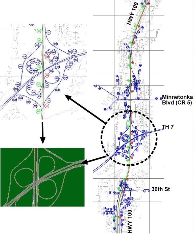
This figure is a link-node diagram of the example freeway system. The diagram on the right shows HWY 100 running north and south. The interchange of HWY 100 and TH7 is enlarged and shown in the upper left portion of the image. The TRAFVU drawing of that interchange is shown in the lower left portion of the image.

Figure 33 . Illustration. Example problem: HWY 100 link-node diagram.

Traffic Demand Data

Traffic demand data for the HWY 100 model was extensive; therefore, a database method for automating the input was essential. With the large number of freeway ramps and arterial intersections, the amount of traffic demand data to be entered for 12-time periods was extensive. The input TRF file for one peak period for this model was nearly 6,000 lines long. Manually entering this much information through TRAFED was judged impractical; therefore, a database method for automating the input was used.

The types of traffic demand data used for this project included:

Arterial volumes were entered as entry volumes at entry nodes and turning percentages at intersections.

Freeway volumes were entered as entry volumes at entry nodes and turn percentages at exit ramps. Additional origin-destination data for mainline freeway were estimated based on traffic counts and likely patterns. There are a number of closely spaced weave areas such as the cloverleaf interchange at TH 7 where none of the entering vehicles will exit at the next exit ramp. The O-D matrices as shown in Figure 34 were used to calculate the origin-destination for each mainline freeway direction. The calculations were converted into TRF format using a database.

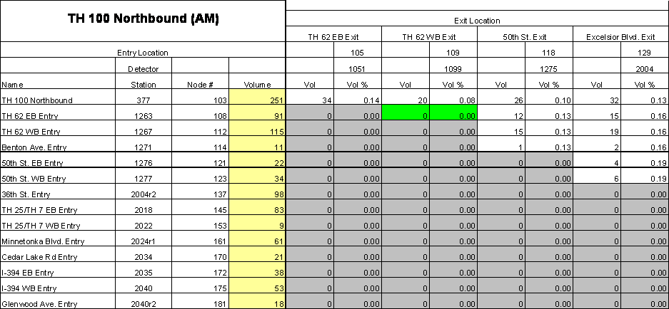
This figure is a table of origin-destination data used in the example study of HWY 100 northbound in the AM time frame. The origin descriptions are shown down the left side of the table. The destination descriptions are shown across the top of the table. The volume and percentage of volume are shown for each origin-destination pair.

Figure 34 . Illustration. Example problem: freeway origin-destination table.

Intersection Traffic Control Data

Traffic signals were actuated, but were coded as pre-timed signals to save time for this example. Data for coding signals was collected by reviewing signals in the field for cycle lengths, phasing, and interval timings and by examining the signal design and timing plans.

Traffic Operations and Management Data

The HWY 100 project was a design evaluation study. Evaluating ITS strategies and incidents were not part of the scope. However, after the design was selected, the final model could be used to test different management scenarios.

Review

After the base model was built and running, the model was checked by comparing QA/QC tables to link-node and coding schematic diagrams and by reviewing the animation. The graphic shown in Figure 35 is a series of screen shots of the HWY 100 Model that was reviewed.

The graphic shown is a series of screen shots of the HWY 100 Model that were reviewed. After the base model was built and running, the model was checked by comparing QA/QC tables to link-node and coding schematic diagrams and by reviewing the animation.

Figure 35 . Illustration. Example problem: base model development review.

1 CORSIM can model random arrivals of pedestrians making a call at an actuated controller which sets the walk signal times. It is coded on the actuated controller at an intersection. The actuated controller pedestrian demand and the vehicle delay are not coordinated in any way. They are input and requested separately and operate independently. Both should be specified when modeling pedestrians at actuated controlled intersections.

Table of Contents | Previous | Next

3.0 Base Model Development

User Node Preferences

Surface Street Node Location

Freeway Node Location

Superelevation, Pavement Friction, and Radius of Curvature

Barriers

Reaction Points

Lane Data

Time Period Varying Demand

Vehicle Entry Headway

Approach 1: Complete Turning Counts or Percentages

Approach 2: Complete Origin-Destination Data

Approach 3: Partial Origin-Destination Data

Minimum Separation of Vehicle Generation

Distribution Among Lanes

Turn Percentages

Interchange origin-destination

Conditional Turn Movements

Origin-Destination Trip Table

Source-Sinks

Clock-time

Demand/Capacity

Speed Control

Multi-threshold Occupancy

ALINEA Control(9)

HOV Bypass Lane

Sign Control

Actuated Signal Control

Pre-timed Control

Right Turn On Red

Signal Optimization

Surface Street Events

Freeway Incidents

Stations

Path

Route

Review

Create a TSIS Project and Set the Run Control Parameters

Link-Node Diagram: Model Blueprint

Traffic Demand Data

Intersection Traffic Control Data

Traffic Operations and Management Data

Review

ALINEA Control⁽⁹⁾