Empirical Studies on Traffic Flow in Inclement Weather

3.0 Research Methodology

This chapter presents a research plan aimed at compiling appropriate data for the analysis of weather impacts on traffic flow behavior and critical traffic stream parameters, namely free-flow speed (u_f), speed-at-capacity (u_c), capacity (q_c), and jam density (k_j). The research plan fuses weather and loop detector data to address two critical issues, namely:

1. Study the impact of precipitation on macroscopic traffic flow indicators over a full-range of traffic states, and
2. Investigate the potential for regional differences in precipitation impacts.

The study analyzes data from three metropolitan areas that cover a wide-range of weather conditions within the U.S. These sites include Baltimore, the Twin Cities, and Seattle. Loop detector data aggregated to a five-minute level of resolution are analyzed as part of the study. In addition, real-time local weather data including precipitation rates are assembled. Utilizing the loop detector data, fundamental diagrams are fit to the data by minimizing a normalized orthogonal error between field observations and model estimates. The optimum free-flow speed, speed-at-capacity, capacity, and jam density are computed for different weather conditions and inclement weather adjustment factors are developed for each precipitation level. Furthermore, statistical models are developed to characterize the behavior of these parameters as a function of the precipitation type and intensity. The procedures developed as part of this project can be easily implemented within the basic freeway procedures of the Highway Capacity Manual (HCM) given that the level of service (LOS) and capacity of a basic freeway segment is characterized using two of the four critical traffic stream parameters, namely: free-flow speed and capacity. It is envisioned that the inclement weather adjustment factor will be applied in a similar fashion to the standard HCM adjustment factors (lane width, lateral clearance, heavy vehicle, etc.) to estimate a final free-flow speed and capacity that is reflective of both traffic and weather conditions.

The steps required for this approach are illustrated in Figure 3.1.

Figure 3.1 Research Methodology Steps

[D]

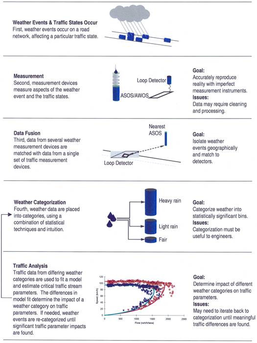
The specifics of the proposed research approach are described in this section. Initially, key traffic stream variables are described. Subsequently, different forms of the fundamental traffic equation are discussed together with the reasoning for selecting the Van Aerde functional form. Subsequently, the statistical techniques that are utilized to analyze the data and develop models that characterize the behavior of critical traffic stream variables as a function of precipitation rates are discussed.

3.1 Key Traffic Variables

Prior to describing the specifics of the research plan, a brief introduction of traffic stream variables is presented to set the stage for the analysis. Traffic stream motion can be formulated either as discrete entities or as a continuous flow. Microscopic car-following models, which form the discrete entity approach, characterize the relationship between a vehicle’s desired speed and distance headway (h) between it and the preceding vehicle traveling in the same lane. Alternatively, traffic stream models describe the motion of a traffic stream by approximating the flow of a continuous compressible fluid. Traffic stream models relate three traffic stream variables, namely:

• Traffic stream flow rate (q) – The number of vehicles that pass a point per unit of time,
• Traffic stream density (k) – The number of vehicles along a section of highway, and
• Traffic stream space-mean-speed (u) – A density weighted average speed (the average speed of all vehicles on a given section of the highway at any given time).

In solving for the three traffic stream variables (q, k, and u) three relationships are required. The first relationship among is inherent in the quantity definition, which states that

[1]

The second relationship is the flow continuity relationship, which can be expressed as

[2]

where S(x,t) is the generation (dissipation) rate of vehicles per unit time and length. This equation ensures that vehicles are neither created nor destroyed along a roadway section.

Both of the above relationships are true for all fluids, including traffic and there is no controversy as to their validity. However, it is the controversy about the third equation, that gives a one-to-one relationship between speed and density or between flow and density, which has led to the development of many fundamental diagrams, also known as first-order continuum models. These models state that the average traffic speed is a function of traffic density. These functional forms describe how traffic stream behavior changes as a function of traffic stream states. Furthermore, they define the values of the critical traffic stream parameters, namely: free-flow speed, speed-at-capacity, capacity, and jam density.

The research plan uses macroscopic traffic stream models to estimate a facility’s free-flow speed, speed-at-capacity, capacity, and jam density during normal and inclement weather conditions. Subsequently, procedures for characterizing inclement weather impacts on traffic stream behavior and critical traffic stream parameters are developed.

3.2 Selected Traffic Stream Model – Van Aerde

Why Traffic Stream Models?

The basic premise of the Lighthill, Whitham and Richards (LWR) theory is a fundamental diagram that relates the three basic traffic stream parameters; flow, density, and space-mean speed. The calibration of traffic stream or car-following behavior within a microscopic simulation model can be viewed as a two-step process. In the first step, the steady-state behavior is calibrated followed by a calibration of the nonsteady state behavior. Steady-state or stationary conditions occur when traffic states remain practically constant over a short time Δt and some length of roadway Δx. The calibration of the steady-state behavior involves characterizing the fundamental diagram that was described earlier and is critical because it dictates:

• The maximum roadway throughput (capacity),
• The speed at which vehicles travel at different levels of congestion (traffic stream behavior), and
• The spatial extent of queues when fully stopped (jam density).

Alternatively, the calibration of the nonsteady state behavior influences how vehicles move from one steady-state to another. Thus, it captures the capacity reduction that results from traffic breakdown and the loss of capacity during the first few seconds as vehicles depart from a traffic signal (commonly known as the start loss). Under certain circumstances, the non-steady-state behavior can influence steady-state behavior. For example, vehicle dynamics may prevent a vehicle from attaining steady-state conditions. A typical example of such a case is the motion of a truck along a significant upgrade section. In this case, the actual speed of the truck is less than the desired steady-state speed because the vehicle dynamics prevent the vehicle from attaining its desired speed. The analysis of such instances is beyond the scope of this study but is provided elsewhere (Rakha and Lucic, 2000; Rakha et al., 2004; Rakha and Ahn, 2004; Rakha and Pasumarthy, 2005).

State-of-Practice Single Order Continuum Models

In selecting the appropriate model for this analysis it is useful to note that traffic models developed over the years have used the same basic variables as those discussed in Section 2. Various functions and relationships have been developed between speed, jam density and/or capacity. Later research attempted to look at differences in driver behavior; specifically the fact that some drivers tend to leave less separation in congested conditions.

Further research on each of the above single regime models revealed deficiencies over some portion of the density-range. The most significant problem that these model development efforts have not solved is their inability to track the measured field data near capacity conditions (May, 1990). This led several researchers to propose two- and multi-regime models with separate formulations for the free-flow and congested-flow regimes.

As a result several multi-regime models have been proposed over the past 40 years. These models developed different formulations depending on the level of congestion with separate formulations for free-flow and congested-flow. Some models included a third category called “transitional flow.” Other models developed identified different relationships for the inside lanes and the outside lanes using the theory that more aggressive higher performance vehicles tend to travel in the left lanes.

While multi-regime models are more advanced than the single-regime models it should be noted that a major disadvantage of multi-regime models are issues related to model calibration. Specifically, the calibration of these multi-regime models is challenging because one needs to identify the cut-points for each of the model regimes and identify which regime field observations fall into.

Figure 3.2 illustrates two sample fits to field observed data for five domains: the speed-flow, speed-density, density-flow, speed-headway, and speed-travel time domains. A visual inspection of the figure provides some good insight into model calibration.

Figure 3.2 Van Aerde and Newell Model Fit to Freeway Data
(Data Source: May, 1990; page 292)

[D]

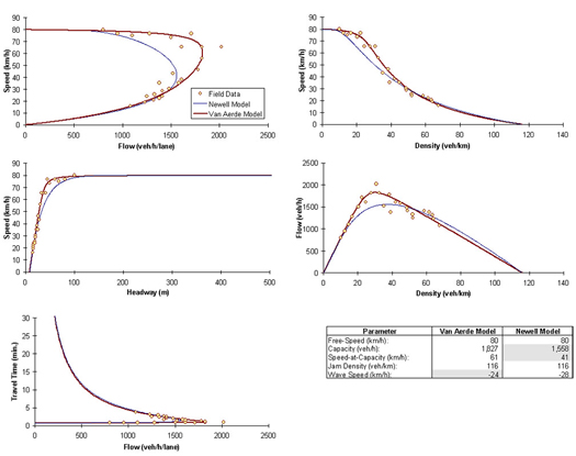
Table 3.1 summarizes the effectiveness of various models in estimating key parameters.

• First, an accurate estimation of the critical traffic stream parameters (u_f, u_c, q_c, and k_j) hinges on a good functional form.
• Second, a functional form that provides a good or reasonable fit in one domain does not necessitate a good fit in other domains. For example, the Newell model provides a reasonable fit in the speed-headway and speed-density relationships; however does a poor job in the speed-flow domain.
• Third, it is difficult to produce a good fit for all traffic states. For example, the Newell model provides a good fit for minimal and maximal flow conditions (free-flow speed and jam density); however the quality of the fit deteriorates as traffic approaches capacity. Table 3.1 also demonstrates that the Van Aerde functional form provides sufficient degrees of freedom to produce a good fit for all traffic states across the various regimes and domains. A brief description of the Van Aerde model is provided in the following section. The quality of traffic stream parameter estimation is clearly demonstrated in Table 3.1. The results for all models except the Van Aerde model that are presented in Table 3.1 were obtained from May (1990) and demonstrate that apart from the Van Aerde model, all single- and multi-regime models do not provide a good estimate of the four traffic stream parameters. Consequently, the Van Aerde functional form will be used to estimate the four critical traffic stream parameters.

Table 3.1 Comparison of Flow Parameters for Single-Regime, Multiple-Regime Models, and Proposed Model

Type of Model	Model	Free-Flow Speed (km/h)	Speed-at-Capacity (km/h)	Capacity (vph/lane)	Jam Density (veh/km)
Valid Data Range [3]	Valid Data Range [3]	80-88	45-61	1,800-2,000	116-156
Single-Regime	Greenshields	91 [outside the valid data range for specified parameter]	46	1,800	78 [outside the valid data range for specified parameter]
Single-Regime	Greenberg	∞ [outside the valid data range for specified parameter]	37 [outside the valid data range for specified parameter]	1,565 [outside the valid data range for specified parameter]	116
Single-Regime	Underwood	120 [outside the valid data range for specified parameter]	45	1,590 [outside the valid data range for specified parameter]	∞ [outside the valid data range for specified parameter]
Single-Regime	Northwestern	77 [outside the valid data range for specified parameter]	48	1,810	∞ [outside the valid data range for specified parameter]
Single-Regime	Newell	80	41 [outside the valid data range for specified parameter]	1,558 [outside the valid data range for specified parameter]	116
Multi-Regime	Edie	88	64 [outside the valid data range for specified parameter]	2,025 [outside the valid data range for specified parameter]	101 [outside the valid data range for specified parameter]
Multi-Regime	2-Regime	98 [outside the valid data range for specified parameter]	48	1,800	94 [outside the valid data range for specified parameter]
Multi-Regime	Modified Greenberg	77 [outside the valid data range for specified parameter]	53	1,760 [outside the valid data range for specified parameter]	91 [outside the valid data range for specified parameter]
Multi-Regime	3-Regime	80	66 [outside the valid data range for specified parameter]	1,815	94 [outside the valid data range for specified parameter]
Van Aerde Model	Van Aerde Model	80	61	1,827	116

Source: May, 1990 pages 300 and 303.

Van Aerde Model

The functional form that is utilized in this study is the Van Aerde nonlinear functional form that was proposed by Van Aerde (1995) and Van Aerde and Rakha (1995). The model bases the distance headway (km) of a vehicle (n) on:

• The speed of vehicle n (km/h);
• The facility free-flow speed (km/h);
• A fixed distance headway constant (km);
• A variable headway constant (km²/h); and
• A variable distance headway constant (h^-1).

This combination provides a linear increase in vehicle speed as the distance headway increases with a smooth transition from the congested to the uncongested regime. This combination provides a functional form with four degrees of freedom by allowing the speed-at-capacity to differ from the free-flow speed or half the free-flow speed, as is the case with the Greenshields model. Specifically, the equation provides the linear increase in the vehicle speed as a function of the distance headway, while the third parameter introduces curvature to the model and imposes a constraint on the vehicle’s speed to ensure that it does not exceed the facility free-flow speed through the use of a continuous function.

Ignoring differences in vehicle speeds and headways within a traffic stream and considering the relationship between traffic stream density and traffic spacing, the speed-density relationship can be derived as a function of the traffic stream density (veh/km) and the traffic stream space-mean speed (km/h) assuming that all vehicles are traveling at the same average speed (by definition given that the traffic stream is in steady-state). A more detailed description of the mathematical properties of this functional form can be found in the literature (Rakha and Van Aerde, 1995 and Rakha and Crowther, 2002), including a discussion of the rationale for its structure. [Of interest is the fact the Van-Aerde Equation reverts to Greenshields' linear model, when the speed-at-capacity and density-at-capacity are both set equal to half the free-flow speed and jam density, respectively (i.e. u_c=u_f/2 and kc=kj/2). Alternatively, setting uc=uf results in the linear Pipes model given that .]

Table 3.2 illustrates the critical traffic stream parameter estimates using the Van Aerde functional form for a number of facility types, demonstrating the flexibility of the model.

Table 3.2 Estimated Flow Parameters for Various Facility Types

Source	Facility Type	No. Obs.	Free-Flow Speed (km/h)	Speed-at-Capacity (km/h)	Capacity (veh/h/lane)	Jam density (veh/km/lane)
May 1990	Freeway	24	80.0	61.0	1,827.0	116.0
May 1990	Tunnel	24	67.5	33.8	1,262.5	125.0
May 1990	Arterial	33	45.0	22.5	581.5	101.9
Orlando	I-4 Fwy	288	87.0	75.5	1,906.3	116.0
Toronto	401 Fwy	282	105.6	90.0	1,888.0	100.0
Amsterdam	Ring Road	1,199	99.0	86.3	2,481.3	114.7
Germany	Autobahn	3,215	160.0	105.0	2,100.0	100.0

Model Calibration

The calibration of macroscopic speed-flow-density relationships requires identification of a number of key parameters, including the facility’s capacity, speed-at-capacity, free-flow speed, and jam density.

This section describes the proposed method for calibrating steady-state car-following and traffic stream behavior using the Van Aerde steady-state model, which is described elsewhere in the literature (Van Aerde, 1995; Van Aerde and Rakha, 1995). The Van Aerde functional form is selected because it offers sufficient degrees of freedom to capture traffic stream behavior for different facility types, which is not the case for other functional forms. Van Aerde and Rakha (1995) presented a calibration procedure that has been enhanced to address field application needs. The technique considers macroscopic speed, flow, and density as dependent variables, and that relative errors in speed, density, or volume of equal magnitude should be considered to be of equal importance. The technique involves the optimization of a quadratic objective function that is subject to a set of nonlinear constraints. This optimization, which requires the use of an incremental optimization search, is demonstrated for several sample and field data sets. The results are compared to several previous analyses that also attempt to fit a linear or nonlinear relationship between the independent variable density and the dependent variable speed. An extensive review of the historical difficulties associated with such fits can be found in the literature (May, 1990).

It is common in the literature to utilize the traffic stream space-mean speed as the dependent variable and the traffic stream density as the independent variable in the calibration of speed-flow-density relationships. However, such a regression fit can only be utilized to estimate speed from density given that the regression minimizes the speed estimate error. To overcome this shortcoming, a concept of fitting a relationship between speed, flow, and density, which does not consider one variable to be more independent than another was considered. The calibration of macroscopic speed-flow-density relationships requires identification of a number of key parameters, including the facility’s expected or mean four parameters, namely; capacity (q_c), speed-at-capacity (u_c), free-flow speed (u_f), and jam density (k_j). The overall calibration effort requires that four decisions be made, namely:

1. Define the functional form to be calibrated;
2. Identify the dependent and the independent variables;
3. Define the optimum set of parameters; and
4. Develop an optimization technique to compute the set of parameter values.

A heuristic tool was developed (SPD_CAL) and described in the literature to calibrate traffic stream models (Rakha and Arafeh, 2007). The procedure can be summarized briefly as follows:

• Aggregate the raw data based on traffic stream density bins in order to reduce the computational space;
• Initialize the four traffic stream parameters u_f, u_c, q_c, and k_j;
• Construct the model functional form and move along the functional form incrementally to compute the objective function. The accuracy of the objective function computation and the computational speed will depend on the size of theincrements used;
• Vary the four parameters between minimum and maximum values using a specified increment;
• Construct the model functional form for each parameter combination and move along the function form incrementally to compute the objective function. Note that the computational accuracy increases as the iteration number increases;
• Compute the set of parameters u_fⁱ, u_cⁱ, q_cⁱ, and k_jⁱ that minimize the objective function;
• Compute minimums and maximums for each variable at specified increments; and
• Go to step 3 and continue until either the number of iterations is satisfied or the minimum change in objective function is satisfied.

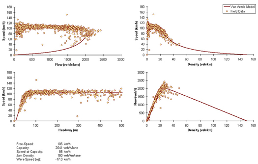
The fit to five-minute data from the Twin Cities, Minnesota, demonstrates that the calibration tool is able to capture the functional form of the data, as illustrated in Figure 3.3. The figure clearly demonstrates the effectiveness of the proposed calibration tool together with the Van Aerde functional form to reflect steady-state traffic stream behavior on this facility over multiple regimes.

Figure 3.3 Van Aerde Model Fit to Freeway Data (Twin Cities, USA)

3.3 Data Analysis and Model Development

The first step in the data analysis will be to obtain a subset of reliable data for processing, by screening the data as follows:

1. Incident data will be removed from the dataset so that the dataset only includes data during incident-free conditions;
2. Detectors in the merging lanes and weaving sections will be removed from the data processing;
3. Using the weather data, the loop detector data will be grouped into different categories. For example, data may be grouped based on the intensity of precipitation. Data from multiple days may be grouped together to ensure that data cover a significant range of traffic states; and
4. Data will be screened for any missing and unrealistic data.

The processed data will be used to study:

• The impact of precipitation on macroscopic traffic flow indicators over a full range of traffic states.
• The impact of precipitation on macroscopic traffic flow indicators using consistent, continuous weather variables.
• The impact of precipitation on macroscopic traffic flow indicators on a wide range of facilities.
• Regional differences in reaction to precipitation.
• Macroscopic impacts of reduced visibility.

Impacts of Precipitation

The short-term direction of the research, as defined by the first four research questions described earlier deal with answering how precipitation affects driving, as a factor of: 1) Traffic State, 2) Intensity, 3) Facility, and 4) Region. The fifth research question addresses the affect of visibility on driving. In order to study the impacts of precipitation on traffic flow and precipitation intensity, the optimum four traffic stream parameters (free-flow speed, speed-at-capacity, capacity, and jam density) will be calibrated for a number of days. A distribution of typical parameter values will be constructed. Depending on the number of inclement weather conditions and the range of states that the inclement weather conditions cover, either a single or multiple repetitions of the data may be available for each site. The distribution of each parameter for the base conditions (ideal weather) will then be compared to the inclement weather parameters. Subsequently, t-statistics will be used to test if the mean parameter values are statistically different. In addition, analysis of variance (ANOVA) tests will be conducted on the data to identify any potential statistical differences for various parameters, including weather, regional differences, and the combination of both weather and regional differences. Figure 3.4 illustrates a sample functional relationship for ideal and inclement weather conditions. The figure also summarizes the key four parameter estimates for both instances and computes a multiplicative inclement weather adjustment factor. The statistical tests that will be conducted will investigate if these adjustment factors are statistically significant, or within the range of typical daily variations.

Figure 3.4 Impact of Precipitation on Traffic Stream Behavior and Parameters

[D]

The first two research issues:

1. The impact of precipitation on macroscopic traffic flow indicators over a full range of traffic states; and
2. The impact of precipitation on macroscopic traffic flow indicators using consistent, continuous weather variables

will be addressed within the context of the analysis procedure shown above. Different states of congestion can be defined along different portions of the curves. Additional curves can be defined based on the characteristics of weather events, with categories based on precipitation type and intensity. These sets of curves can ultimately be utilized to define different adjustment factors as shown in Table 3.3.

Table 3.3 Hypothetical Capacity Adjustment Factors

Congestion State	Weather State: Clear	Weather State: Light to Moderate Rain	Weather State: Heavy Rain	Weather State: Light Snow	Weather State: Heavy Snow
Uncongested	1.0	0.95	0.85	0.9	0.75
Transitional	1.0	0.90	0.7	0.8	0.55
Congested	1.0	0.75	0.55	0.6	0.40

Statistical Analysis

Crow et al. (1960) state that “the data obtained from an experiment involving several levels of one or more factors are analyzed by the technique of analysis of variance. This technique enables us to break down the variance of the measured variable into the portions caused by the several factors, varied singly or in combination, and a portion caused by experimental error. More precisely, analysis of variance consists of 1) partitioning of the total sum of squares of deviations from the mean into two or more component sums of squares, each of which is associated with a particular factor or with experimental error, and 2) a parallel partitioning of the total number of degrees of freedom. The assumptions of the analysis of variance (ANOVA) technique are that the dependent variable populations have the same variance and are normally distributed (Littell et al., 1991). Consequently, tests were conducted to ensure that the dependent variables were normally distributed using the Shapiro-Wilk statistic which produces a score ranging from 0 to 1. The closer the score is to 1, the more likely the data are normally distributed.

The distinction between normality and non-normality of data and what should be done in the case non-normality exists are two controversial issues. Some researchers, on the one hand, believe that the ANOVA technique is robust and can be used with data that do not conform to normality. On the other hand, other researchers believe that nonparametric techniques should be used whenever there is a question of normality. Research has shown that data that do not conform to normality due to skewness and/or outliers can cause an ANOVA to report more type 1 and type 2 errors (Ott, 1989). Conover (1980) recommends use of ANOVA on raw data and ranked data in experimental designs where no nonparametric test exists. The results from the two analyses can then be compared. If the results are nearly identical then the parametric test is valid. If the rank transformed analysis indicates substantially different results than the parametric test, then the ranked data analysis should be used. As a result, an approach using both an ANOVA on the normalized data and an ANOVA on rank-transformed data may be utilized depending on the normality of the data. We suggest ranking the data when the Shapiro-Wilk test is less than 0.85.