Weather Applications and Products Enabled Through Vehicle Infrastructure Integration (VII)

6. Case Studies

INVESTIGATING ACTUAL WEATHER-RELATED VEHICLE DATA ELEMENTS

The efficacy of VII-enabled data is illustrated in Figures 6.1 and 6.2. Figure 6.1 displays data from a DaimlerChrysler vehicle operating north of the Detroit downtown area on 16 February 2006. Included in the figure are radar data (base reflectivity) from the Detroit Doppler weather radar valid closest to the time of the vehicle data. Data were available from the vehicle at one-minute intervals, while base reflectivity scans were available on six-minute intervals. The radar data show reflectivity or echo intensity measured in decibels (dBZ), which generally correlates with precipitation rate. Cooler colors indicate lower reflectivity and warmer coolers indicate higher reflectivity. Vehicle data elements include information on wiper state: 0 is off, 13 is low, 14 is high, and 1 through 6 are intermittent settings. Barometric pressure in inches of Mercury (inches Hg) and air temperature in degrees Fahrenheit (oF) are also supplied.

The Automated Surface Observing System (ASOS) located at the Detroit City Airport (DET) reported light rain and misty conditions throughout much of the day on 16 February, with some thunderstorms during the afternoon and evening hours. Temperatures ranged from about 34oF (1oC) in the morning to a high of roughly 55oF (13oC) in the afternoon and evening. Station pressure ranged from approximately 28.90 to 29.40 inches Hg during this time.

Figure 6.1A shows the vehicle driving shortly after noon (17:12Z) on 16 February. At this time, the wiper state is zero, which denotes that the wipers are not in operation. This is consistent with radar reflectivity returns in the area; there are no reported radar echoes in the immediate vicinity of the vehicle. An area of light to moderate reflectivity does exist to the south of the vehicle's location. These echoes are moving to the northeast. An air temperature of 35.6oF (2oC) is reported by the vehicle. This is well correlated with the 33.8oF (1oC) atmospheric temperature reported by the Detroit ASOS (approximately 12 miles southeast of the vehicle's location) station about half an hour earlier. This difference is reasonable, as nearby convection and/or frontal boundary location may be influencing the readings. By 17:58Z (Figure 6.1B), the radar echoes have moved into the vehicle's area. Data from the vehicle indicates that the wipers are on low. Temperature and pressure readings have increased slightly. Figure 6.1C and 6.1D capture the vehicle moving to the northwest along Interstate 75 at 23:25Z and 23:49Z, respectively. In Figure 6.1C, the wipers are on, but the driver is utilizing an intermittent setting. This setting could be the result of very light precipitation in the area, spray from the roadway, or a combination of both. The wiper setting changed to high by 23:49Z, which correlates with the more intense echoes observed by the radar. According to the vehicle data, temperatures have risen between 14-18oF (8-10oC) from those reported some six hours earlier. Again, this is consistent with ASOS data, as was the reduction in pressure reported by the vehicle. This case is promising; it indicates that the vehicle data are consistent with the nearby official surface observations and radar data.

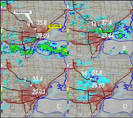
FIGURE 6.1. Vehicle data valid at 17:12Z (A), 17:58Z (B), 23:25Z (C), and 23:49Z (D) on 16 February 2006 overlaid with WSR-88D radar data. Vehicle data include vehicle position (white circle), wiper state (to the upper left of vehicle location), atmospheric temperature (oF) (upper right), and barometric pressure (inches Hg) (lower right). Vehicle data courtesy of DaimlerChrysler.⁶

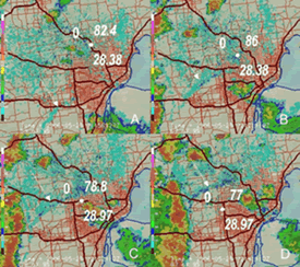
FIGURE 6.2. As in Figure 6.1, except valid times are 21:56Z (A), 22:21Z (B), 22:32Z (C), and 22:41Z (D) on 25 May 2006. Arrow denotes the location of outflow boundary.

Both of these cases demonstrate the benefit of vehicle data in the diagnosis of atmospheric conditions. It is also readily apparent that the proliferation of VII-enabled data would result in information on spatial and temporal scales that would support advances in the analysis and prediction of weather and road condition hazards. For example, in the case of thunderstorm generated outflow boundaries, an adequate number of vehicles would not only aid in identifying the location of the outflow boundary, but would permit additional characterization of the outflow boundary (e.g. scale, structure, etc.). These data can be used to initialize high-resolution numerical weather models, which presently have difficulty analyzing and predicting small-scale structures such as these because there is currently a lack of surface observations on these small-scales.

Weather models today can be run operationally over small domains ( 620 mi by 620 mi [~1000 km by 1000 km]) with horizontal grid spacing as low at 1/2 miles (~1 km). As the grid spacing of weather models decreases the need for high-resolution observations increases as these data are required to initialize and validate the models. As is evident from the cases presented herein, VII-enabled data will help address the need for more observations.