II. Signal Timing Process

There are eight distinct steps that define the signal timing development process. Not every step requires a costly effort to complete in every instance. For example, it is not difficult to determine the signal grouping for an arterial with three signals. However, it may be a somewhat more difficult task to identify signal groupings for 50 intersections in arterial and grid networks. The steps begin with identifying the system boundaries. This boundary helps to minimize the scope-creep temptation of adding just one more intersection. From here the steps are a logical and straightforward process that will enable the Practitioners to efficiently acquire only the essential information. This methodical procedure will enable Practitioners to avoid one of the most costly endeavors—making a second or third trip to the field to obtain more data, or data that was missed this first time.

1 - Identify the System Intersections

Although this step is obvious, it is a necessary first step. The intent is to clearly identify all intersections that will be analyzed in the effort. This is an important issue because all intersections will require a baseline amount of attention at the start of the effort. This effort translates to a cost that we want to minimize.

Each intersection must be identified by a unique name and number. The numbering scheme should be organized in a way that reflects the geometry of the intersections. For example, if the intersections are on an arterial that generally runs east and west, the numbers might start with the lowest number for the western most intersection and increase to the east. Other basic information should be defined at this time including whether the intersection is currently signalized, political jurisdiction, responsible maintenance organization, and any other general, readily-available information or characteristic. This information should be entered into a spreadsheet.

It is important to recognize at this point that this listing is all of the intersections that are under consideration. This does not imply that all of these intersections will necessarily operate together as a group or system; it simply means that these intersections will be considered and evaluated. Some or all may operate together as a single group, two or more may operate as separate groups, or one or more intersections may operate better as isolated intersections. These solutions can only be evaluated after an operational analysis.

2 - Collect and Organize Existing Data

The data needed to prepare signal timing plans can be divided into two categories: descriptive and demand. The descriptive data is the easiest to obtain, and, for the most part, can be obtained from the files of the operating agency. These data include the following:

• A condition diagram of each intersection showing the number of lanes and width of each lane on all approaches. The condition diagram must have a North arrow and show the street names.
• A phasing diagram for intersections with existing controllers. It is important for the phasing diagram to include the NEMA phase number for each phase movement. The phasing diagram must also show all overlaps (if any).
• Existing detector location, type (presence or passage), and phase assignment information. These data are necessary to determine the phase interval settings, such as the minimum green and the extension.
• Existing traffic count data. The most useful data are turning movement counts. When using old counts, it is necessary to determine whether there has been any major change in the traffic demand since the count was made. If there has been no significant change in demand, then the counts can be adjusted for annual traffic growth. If there has been a major change, then the counts may not be as useful. Hourly road tube counts and even Average Annual Daily Traffic 24-hour counts are also useful information and can be used to estimate traffic growth and even estimate turning movement counts. This information may be available from the local jurisdiction, from the local or regional planning agencies, and/or the state department of transportation. Because manual counting is the single most expensive element to signal timing, assimilating existing data is usually well worth the effort and cost.
• Distance between intersections and the free-flow travel speed for the conditions under which the timing plan will operate. This information should be depicted on a map of the area showing the roads and signalized intersections. It is not necessary for the map to be drawn to scale; however, it is important for each link on the map to be long enough to be able to show various data such as link length, speeds, and volume.
• An estimate of the number of different timing plans that may be needed and the times during which each plan would be used. This information must be determined based on the available traffic count data and the experience of the practitioner.

3 - Conduct Site Survey

This step may be the most important step in the process. Although it is possible to generate both local and coordinated signal timing parameters without ever seeing the intersection, this is a very dubious practice. Physical constraints that may or may not be noted on a plan sheet, but that may have an obvious impact on traffic flow, are immediately obvious to the viewer. Vegetation sight distance obstructions, adverse approach grades and curvature, and fading pavement markings are examples of factors that affect traffic flow that are apparent during a site survey.

The site survey is most effective when conducted after all of the existing data has been collected and organized. The purpose of the site visit is to confirm that the existing information gathered in the previous step is accurate and to collect any additional data that may be needed.

It is strongly recommended that each intersection be visited during the hours for which the timing plan is being developed. For example, if four timing plans are being developed, then the intersection should be visited during the peak AM period, during a typical day period, during the peak PM period, and during a low-volume night period. Most of the information will be obtained during the typical day period, but site visits during the extreme conditions of both high and low volume will frequently provide insight into signal operation that cannot be obtained any other way.

The basic intersection checklist includes the following:

Condition Diagram—This may be a verification of the intersection sketch obtained during the previous step, or if there is no existing drawing, preparation of a new diagram. This diagram should include the following:

• Intersection sketch showing driveway curb cuts, sidewalks, crosswalks, North arrow, street names
• Approach lane configurations including widths and movement assignments
• Sight distance restrictions and cause such as vertical or horizontal curvature, and vegetation
• Curb restrictions (e.g., parking, loading zone, transit stop, etc.).

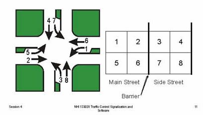
Phasing Diagram—Like the Condition Diagram, this diagram is either a verification of existing information or the preparation of a new document. It is important for the phasing diagram to include the NEMA phase number for each phase movement and to identify the NEMA phase number with the corresponding traffic movement by direction (see Figure 2). For example, Eastbound Left Turn—Phase 5; Eastbound Through—Phase 2. The phasing diagram must also show and identify all overlaps (if any).

Figure 2. Standard 8-Phase Intersection, Layout.

Detector Locations—Existing detector location, type (presence or passage), and phase assignment data are necessary to determine the phase interval settings. The purpose of the field visit is to verify that the detectors are deployed as shown on existing documents; but more importantly, the purpose is to verify that the detectors are operating as designed.

Existing Controller Settings—With modern controllers, it is not unusual to find three distinctly different sets of local controller timing data: the data in the controller itself, the data shown on intersection records in the controller cabinet, and controller data from the office records. Of course, the purpose of the site visit is to reconcile any differences among these record sets and to verify that the settings are reasonable for the traffic conditions.

Traffic Flow Observations—While visiting each intersection, record the typical free-flow speed observed on each link and note this information on the map prepared in the previous step. Notice that the speeds may be different for each timing plan. This observation is important because it will have a major impact on the offset. It is also practical to determine the link length using the vehicle’s odometer to verify the information recorded on the map. This independent verification of link length could save a great deal of work that would be required if the distance recorded on the map were wrong.

For this minimum cost approach to signal timing to be effective, it is vitally important to make full use of all existing information. At this point in the process, the Practitioner will be able to observe the operation of the intersection during the time period of interest with full knowledge of the existing parameters and detector operation. While it would be valuable to be able to use an analytical tool to evaluate intersection performance, the low-budget approach cannot support this luxury. Instead, the observations and experience of the Practitioner are substituted.

4 - Obtain Turning Movement Data

This step involves the preparation of turning movement data for each Primary intersection for each timing plan to be developed. The following options are available to the Practitioners to acquire these data listed in descending order of expected accuracy:

1. Conduct a new turning movement count for the period in question.

2. Conduct a “Short Count” using the procedures discussed in the following section.

3. At an intersection where there has been no significant construction or development, update an old turning movement count to reflect general traffic trends.

4. Estimate turning movement data using the methods discussed in the following section that are based on NCHRP 255, “Highway Traffic Data for Urbanized Area Project Planning and Design.” This effort may be performed using the program TurnsW, which estimates turning volumes from existing link volumes.²

5 - Calculate Local Timing Parameters

As previously noted, it is not unusual to find conflicting information concerning controller parameters among the various record sets in the office and in the field. It is assumed that the field observations have identified a situation whereby the local controller settings require a revision to improve the intersection performance. This step represents the work necessary to revise existing local controller operation parameters.

The local operation parameters are the settings, such as phase minimums, maximums, change, and clearance intervals. These settings are primarily a function of traffic demand, the geometric design of the intersection, and the type and location of detectors.

6 - Identify Signal Groupings

At this point in the signal timing process, all of the intersections should be operating efficiently as isolated intersections. In other words, each intersection should be processing the local demand. Of course, operating efficiently as an isolated intersection and operating efficiently as a system are two entirely different situations.

The purpose of this step is to identify groups of signalized intersections that should operate together as a coordinated unit. One constraint of grouping signals is that all controllers in a group must operate on the same cycle length. It is likely that the cycle length requirements for different intersections are not always identical. A trade-off of coordinated operation is that some of the intersections in a group will operate at an inefficient cycle length. This negative must be more than offset by the benefits derived from coordinated operation.

7 - Calculate Coordination Parameters

In contrast to the local operation parameters, which can number over one hundred when the parameters for each phase are counted, the number of coordination parameters is limited to cycle length, offset, and split (phase force-off). There is one combination of these parameters for each timing plan.

To develop these parameters, the Practitioner is faced with two basic options: to use a computer model, such as PASSER™ or Synchro, or to use the manual methods. It is important for the traffic signal engineer to know the manual methods because they provide the means to conduct independent checks of the computer models. For all practical purposes, however, most signal timing is done with computer optimization models.

The minimum cost approach assumes that some model input parameters may be estimated. It is important to note that it is always better to measure or observe the parameter. Fortunately most programs provide a method to lock some timing parameters while allowing the software to optimize others. For example, at minor intersections the durations of the minor phases (left turn and side street movements) may be determined manually and then input into the model.

When a computer model is available, it is advisable to use the program for several reasons:

1. Much of the input required for both manual and computerized methods is associated with the description of the network. This includes parameters like signal phasing, link distances and speeds, and intersection geometrics. With a computerized approach, this information can be readily leveraged into generating new timing plans with relatively few changes in the input.

2. The data structure of the model will ensure that key information is not overlooked.

3. The data files provide documentation for both the input and the output.

8 - Install and Evaluate New Plans

The final step in the process is to install and evaluate the new timing plans in the field. There are two basic analytical procedures available to the Engineer to evaluate new timing plans: stopped-time delay studies and moving car travel time studies. With a shoestring budget, it is unlikely that either of these techniques can be employed. Because the shoestring budget approach has skipped many steps that normally provide checks and balances, we recommend that the Engineer use special care when using these plans for the first time. Specifically, we recommend the following:

1. Install the signal timing parameters in each controller.

2. During a benign traffic period, such as mid-morning after the AM rush hour, put the plan in operation and observe that the offsets are as expected. Check the operation at every intersection.

3. Place the plan in operation during the period for which it was developed. Again observe the offsets at each intersection. During peak periods, check left turn bays for spill-back. Make minor adjustments as necessary.

This effort should not be minimized; the practitioner should expect to spend 20 to 30 percent of the timing budget on this evaluation and “fine-tuning” effort.

 

 

2 “TurnsW” is a computer program developed by Dowling and Associates.