FHWA Freight BCA Study:
Summary of Phase II Results
Prepared by
ICF Consulting
9300 Lee Highway
Fairfax, Virginia 22031
703-934-3000
- and -
HLB Decision-Economics
8403 Colesville Road, Suite 910
Silver Spring, Maryland 20910
301-565-0391
Under subcontract to: AECOM
January 2004
Contents
- Introduction
- Benefits of Highway-freight Improvement: The Problem
- Method: The Analytical Approach to the Problem
- Next Steps
1. Introduction
This summary report presents the results of Phase II of FHWA's Freight Benefit-Cost Study. The purpose of Phase II is to establish the long-term benefits of highway-freight improvements by examining the dynamic interactions between freight transportation demand, transportation costs, and the condition and performance of the Nation's highway system. The Phase II Report, delivered to FHWA under a separate cover, assesses these interactions beyond the traditional travel-time savings within the conventional benefit-cost analysis framework. That is, the methodology adopted allows for the quantification of the effects of transportation system improvements in relation to (1) immediate cost reduction to carriers and shippers, (2) the impact of improved logistics while keeping output fixed, and (3) additional gains from re-organization such as increased demand, new or improved products.
While the Phase II Report documents the results of the quantitative analysis in a rigorous manner, the goal of this document is to summarize those results in a manner that is more accessible to non-economists. Consequently, this document is organized into four sections (including this introduction). The following section describes the measurement challenge that is the subject of Phase II. Section 3 describes the statistical analyses that were conducted to measure the full effects of freight transportation improvements. Section 4 discusses next steps.
2. Benefits of Highway-freight Improvement: The Problem
| Box 1: Specifically, conventional benefit-cost analysis tools do not capture the unique effects of improvements to our freight transportation systems on economic productivity. Yet, if we think of freight transport as a necessary input in the production of goods and services (e.g., manufacturers must move their product from a production site to a consumption site, or market), then the benefits of freight improvements become clearer.
|
Measured by value or by tonnage, more freight moves over the highways than by any other mode. It is highly desirable, then, that decision makers and planners at all levels of government know the amount of the economic benefits that flow from improvements in highway-freight carriage (originating from both infrastructure and infostructure investments); but, in fact, they do not know this. In the past decade or so, considerable strides have been made in the measurement of the benefits to passengers from highway improvements. FHWA's own Highway Economic Requirements System (HERS) is one example. Other models, such as StratBencost, have been developed for analysis at the project level. These models take account of trucks as part of the traffic stream but benefits to goods-carrying trucks are counted only in a limited way. Changes in costs of operating trucks, including changes in labor costs, that stem from increased speeds are counted. But the productivity-enhancing contributions of improvements in the freight system are not counted.1
This is a major omission. Changes in speed and reliability have significant effects on shippers (see Box 1); the full economic benefits of highway-freight improvements are not known unless these effects on shippers are explicitly treated in the analysis. The purpose of FHWA's Freight Benefit-Cost Analysis (BCA) Study is to develop a method for analyzing and estimating the value of these effects. The ultimate goal is a method that would allow planners and analysts to calculate a "mark-up" factor that could be used with existing benefit-cost models to estimate the full benefits of highway-freight improvements. This factor would be a percentage increase by which the benefit estimate from a model such as HERS or StratBencost would be increased to reflect the full benefit from an improvement in highway freight movement. When fully developed, such a factor would allow planners to adjust it for conditions specific to a particular project and corridor-for percentage of combination trucks in the vehicle flow, for example. The purpose of Phase II of FHWA's study is to advance the development of a method that will enable us to estimate the mark-up factor.
Logistics and the Demand for Freight Transportation
| Box 2: Strictly speaking, shippers, (i.e., the owners of the cargo) when deciding on how to best get their products from production centers to markets, look at generalized logistics costs. Simplistically, the elements of logistics costs are 1) transportation costs, 2) the costs of carrying inventory, and 3) the costs associated with product storage facilities (such as warehouses or distribution centers). Generalized logistics costs are what shippers strive to minimize given other production inputs and total logistics costs comprise transportation, inventory, and storage (costs of warehouses, insurance, etc.). Historical data on transportation and total logistics costs, as seen in the graph below, show that transportation has steadily increased as a share of total logistics spending over the period since 1980-a period in which truckload trucking and rail rates were steadily falling in real terms. This illustrates the "reorganization effect" in which logistics set-ups are revamped; transportation spending is substituted for inventory cost with reduced logistics costs per unit as a result.
|
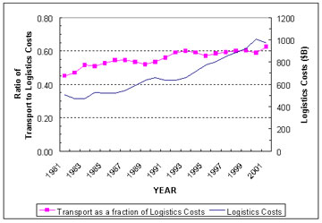
Exhibit 1 shows, in capsule form, the benefits that flow from an improvement in freight movement. The approach we have developed measures the first and second-order benefits. It does not necessarily capture the third-order benefits-benefits from improvements in product quality or new products. It does not address "other effects" at all. These effects, such as changes in regional employment or income, are of great interest to local or State officials, but, under the strict rules of benefit-cost analysis, may not be treated as benefits in addition to the transport-efficiency benefits we seek to measure.
| Exhibit 1: Effects of Improved Freight Transportation | |
|---|---|
| First-order Benefits | Immediate cost reductions to carriers and shippers, including gains to shippers from reduced transit times and increased reliability. |
| Second-order Benefits | Reorganization-effect gains from improvements in logistics. Quantity of firms' outputs changes; quality of output does not change. |
| Third-order Benefits | Gains from additional reorganization effects such as improved products, new products, or some other change. |
| Other Effects | Effects that are not considered as benefits according to the strict rules of benefit-cost analysis, but may still be of considerable interest to policy-makers. These could include, among other things, increases in regional employment or increases in rate of growth of regional income. |
First-order benefits2 are those that shippers realize while making little or no change to their conduct of business, other than some downward adjustment in safety stocks; these benefits are limited to the initial cost savings. But firms will not leave their business operations unchanged when there are changes in the cost and quality of a significant input. Beyond a reduction in trucking costs,3 shippers will receive direct benefits as reduced congestion increases speed and reliability. Greater speed (lower transit times) increases the "reach" of any particular facility such as a factory or distribution center. Greater reliability of delivery times lets companies reduce safety stocks of goods that they need to hold as buffers against failed deliveries and otherwise may allow leaner inventories in the supply chain.
Faced with some combination of lower truck rates, increased speed, and increased reliability, firms will reconsider the amount of freight transportation they buy (see Box 2). In particular, this will take the form of reviewing basic logistics arrangements-number and spacing of distribution centers for example.4 If fewer, more widely spaced warehouses can serve the same set of retail outlets or customers, a firm will be able to reduce inventory costs and increase its sales. The reduced real cost of freight transport lets a company buy more freight transport and reduce its inventory costs, thus reducing total logistics costs even though spending more on transportation. The resulting efficiency gain results in reduced unit costs and increased output.
3. Method: The Analytical Approach to the Problem
| Box 3: To estimate the effects of improvements in the freight highway system (via both infra- and inforstructure), the primary relationship that we seek to understand is how the demand for trucking changes as the volume-to-capacity (V/C) ratio (or delay) changes.
In addition, to capture indirect effects, the relationship that we need to understand is how truck rates vary as V/C ratio (or delay) varies.
|
The economic theory underlying the approach is summarized in the Phase II Report and fully described in the reports prepared under Phase I of the FHWA BCA Study. Details of the statistical analysis and its results are also presented in subsequent sections of this report. Here, we set out the principles of the economic theory and explain how those principles were applied in the statistical analysis.
In economic terminology, the method is based on estimating the demand for highway-freight transport. In non-economic terminology, this means the method is based on measuring the degree of shippers' response to improved highway performance and lower truck rates. By shippers' response, we mean the change in the amount of highway-freight carriage they buy.
The underlying economic principle here is that buyers of a good reveal the degree of benefit they get from a price reduction by the amount to which they increase their purchases of the good in question. If they buy a lot more of the good, then that is a clear signal that they are getting a significant additional benefit. A slight increase in purchases indicates limited additional benefit from the price reduction. In order to quantify benefits, we need to find a way to measure these responses. We do this with statistical analysis.
For the purpose of statistical analysis, we need to formulate equations (in economic terminology, demand equations) that express the relationship between quantity purchased and price. In the transportation context, we often think of price as some combination of money price and time costs (i.e., transit time and reliability). Basically, we are looking for shippers' responses to changes in the performance of the highway system. For this purpose, we may use the volume/capacity (V/C) ratio as a measure of highway performance. The V/C ratio is a convenient way of expressing congestion level in a single measure. Further, enough empirical work has been done to allow conversion of a V/C ratio to congestion-induced delay.5, 6
The effects of a change in highway performance will come to a shipper in two ways, an indirect way and a direct way. The indirect way is through changes in truck rates. Changes in highway performance will affect carriers' costs and that effect will be reflected in changes in carriers' prices. But shippers will also be affected directly. Changes in speed and reliability will have impacts on shippers in addition to those from changed truck rates. Therefore, we need to examine the responses of freight-transport buyers both to changes in highway performance and to changes in trucking rates.
We developed, accordingly, two equations for the statistical tests (see Box 3 on the previous page): the trucking-rate equation and the trucking-demand equation. The trucking-rate equation relates changes in trucking rates to changes in highway performance; the trucking -demand equation relates changes in highway freight-movement to changes in truck rates and changes in highway performance. Highway freight movement is measured by freight VMT (i.e., miles traveled by freight-hauling trucks)-in other words, the amount of freight movement actually bought by shippers (including private carriage).
The economic logic in these two equations (which are described fully in the Phase II Report) is comparatively simple and straightforward. The task of using them in statistical analysis is far from simple. The difficulty we face is that we are trying to isolate the effect of highway performance on trucking rates and on shippers' demand for highway freight-movement. In either case, the driving issue is whether or not highway performance is a significant force given everything else that affects trucking rates and the demand for trucking (e.g., fuel prices, the economy, etc.). We know it has an effect, but we have to try to separate that effect from other stronger forces. 7
Data Used in the Analysis
| Box 4: The freight corridors included in the analysis are listed below.
Corridors were selected from FHWA's list of 70-plus significant freight corridors. Relatively short-segment corridors were selected to ensure distinctive highway performance characteristics, and corridors where roadway performance matters were chosen to capture effects of congestion. |
Two basic approaches were tried in the statistical work, cross-section analysis and analysis with panel data. Cross-section analysis entails comparison of the data across all the corridors in a single year, (1998 in this case) with no analysis across time. With panel data, observations across selected corridors (see Box 4) over time from 1993 to 2000 were analyzed.
The statistical analysis was designed to work with readily available data. Any attempt to do otherwise would have multiplied, many folds, the resources and time required for this work. Full details on all data used and the sources are set out in the Phase II Report. Here, we need to describe the principal data elements and their sources. The principal data elements are truck flows, V/C ratios, and trucking rates in selected corridors and over time. It is necessary to use data from a number of corridors, so we can observe how trucking rates and the demand for trucking vary under different conditions of highway performance; data over time are required for the same reason. The only way that statistical analysis can work is through observation of the key variables under differing conditions.
Volumes of truck traffic and V/C ratios were taken from the HPMS database. In each corridor there are a number of HPMS segments. Annual average daily traffic (AADT) counts are available for each HPMS segment together with the percentage of combination trucks in the vehicle mix. These data were used to derive freight truck-miles for each corridor. Similarly, an average of segment V/C ratios, weighted by segment length, was used to derive V/C ratios by corridor. For part of the statistical analysis, where a time series was not used (i.e., for the cross-section analysis), data from FHWA's Freight Analysis Framework (FAF) on truck flows and V/C ratios were used. FAF provides these data for 1998.
Also, for the cross-section analysis, trucking rates were taken from posted rates of less-than-truckload (LTL) companies for trips between the endpoints of a specific corridor. LTL rates were used because they are publicly available from each major carrier. For time-series rate data, rates from a rate bureau were used.8 We recognize that posted rates do not reflect discounts that are negotiated with large customers. But, for this analysis, we assumed the variation of rates among corridors or across time accurately reflects relative rates. For this analysis, it is the ratios among rates in different corridors and times, not the absolute rates, which matter.
Results of Statistical Analysis
Numerous variations of the relationships that are presented in Box 3 (above) were explored in the statistical work that was conducted as part of this study, and each is presented in the Phase II Report. Generally, speaking, the results of the statistical analysis come in the form of parameters that give specificity to the equations we are analyzing. In a mathematical sense, the results come in the form of numbers (coefficients on the variables in the equations) that put the relationships in definite, quantitative terms. For example, the coefficients in the trucking-rate equation would state the degree to which trucking rates respond to changes in highway performance. The coefficients in the trucking-demand equation would state the degree to which truck-miles vary with trucking rates and highway performance.
We used two kinds of tests when we evaluated the usefulness of statistical results.
- First, do the results make any sense? In the first test, we asked ourselves whether the coefficients make sense intuitively. Consider the trucking-demand equation. If the coefficients tell us that, after accounting for all other relevant factors, firms buy more highway freight movement when trucking rates rise and congestion gets worse, then we know we have not succeeded in isolating the effects of trucking rates and congestion on the demand for trucking services. We might have failed for all sorts of technical, statistical reasons or for reasons relating to data quality and/or comprehensiveness (e.g., not enough data, poor quality of the data, etc.).
- Second, should we believe the results? In asking whether we should believe the estimates, we applied a number of statistical tests that measure the validity or strength of the statistical relationships being reported. These tell us the degree to which we can accept the coefficients as accurate.
As discussed earlier, two types of statistical analyses were undertaken to investigate the effects of highway performance on the demand for trucking and on trucking rates: 1) a cross-sectional analysis that draws on data across 30 corridors for 1998 and 2) a cross-sectional and time-series (panel data) analysis that builds on the cross-sectional database by including historic data on all of the relevant variables.
Cross-Sectional Analysis
| Box 5: The cross-sectional analysis did not work. Three sets of analyses were conducted based on different approaches to defining corridors. But in every case the statistical relationships between highway performance and the demand for trucking, or trucking rates that we were seeking to define were counter-intuitive or insignificant.
|
The results of the cross-section analysis were not usable for the trucking-demand and the trucking-rate equations (see Box 5). Numerous alternatives for structuring the analysis were tested, but none provided results that could be used. For example, estimated coefficients suggested that rising trucking rates and rising congestion would induce shippers to buy more highway-freight movement, which is counter to what we had set out to prove (i.e., that improvements in the freight system led to a re-organization of logistics that resulted with higher levels of freight transport demand).
Panel Data Analysis
The statistical analysis that was conducted with a panel data set provided useful results for the trucking demand equation, but not for the trucking-rates equation. In the case of the trucking-rates equation, results from the panel data analysis showed that, other things being equal, increasing levels of congestion would reduce freight charges. Possible explanations for such counter-intuitive results include:
- Data availability problems: only Less-than-Truck-Load (LTL) rates were available on a time series basis;
- Data quality problems: large and seemingly inexplicable variations in congestion indices were found in HPMS; variations in segment length and segment selection were also found along some of the sample corridors;
- Specification problems: the freight rate equation we were trying to estimate does not explicitly account for the supply of truck shipping services in the sampled corridors. What the results may be capturing is the fact that highly traveled corridors are also those where competition among truckers is more intense, leading to lower shipping rates. Various measures of economic activity, and truck traffic itself, were used as explanatory variables in an attempt to control for such effects, but the results that isolate the effects of measures of highway performance on trucking rates were still counter-intuitive.
However, in the case of the trucking-demand equation, the panel data yielded useful results. In that case, the estimated coefficients showed that lowering the V/C ratio would lead to an increase in truck miles; it showed the same result when the V/C ratio was converted to a measure of delay (i.e., as delay goes down, demand for highway freight goes up).
Exhibit 2 provides a summary of findings regarding the impact of changes in highway performance on the demand for trucking using panel data and three different statistical approaches (see the Phase II Report for a description of those approaches and for definitions of the statistical terminology referenced in the table).
| Exhibit 2: Estimated Impact of Changes in Highway Performance on Freight Demand | ||
|---|---|---|
| Model / Reference | Implied Relationship Between the Demand for Trucking and the Measure of Highway Performance | Interpretation |
| Pooled Regression Trucking Demand as a function of Delay per Mile and a number of other control variables. |
-0.0072 | Other things being equal, a 10% decrease in delay per mile increases the demand for trucking by 0.07%. |
| Fixed Effects (to improve reliability
and robustness of estimated relationships) Trucking Demand as a function of Delay per Mile and a number of other control variables. |
-0.0102 | Other things being equal, a 10% decrease in delay per mile increases the demand for trucking by 0.1% (or a tenth of a percent). |
| Fixed Effects (to improve reliability
and robustness of estimated relationships) Trucking Demand as a function of the V/C Ratio and a number of other control variables. |
-0.0849 | Other things being equal, a 10% decrease in the V/C ratio increases the demand for trucking by almost 1%. |
Although these results should be interpreted with some caution given the difficulties and data limitations encountered in the course of this project, the estimated impact ranges from a 0.07 percent to 1.00 percent increase in the demand for trucking (measured by average daily truck traffic) for every 10 percent decrease in measured congestion (measured by delay and/or the V/C ratio). So, based on this analysis, a highway improvement leading to a 10 percent decrease in measured congestion-from a V/C ratio of 0.60 to a V/C ratio of 0.54, for example-would increase truck movements along the improved highway segment by about 1.0 percent.
The overall result is that the effect we sought to measure, the impact of highway-performance improvement on shippers, is real and is measurable. Moreover, the results were sufficient to permit a preliminary estimate of a mark-up factor; an approximation of the percentage by which benefits found in available benefit-cost models should be increased to reflect freight benefits. These preliminary estimates were in the range of 14.7 to 15.9 percent.
4. Next Steps
We see two immediate applications of the findings reported here. One pertains to FHWA's policy analysis and planning function on behalf of Congress. The second pertains to planning at the state and local level.
- Our first recommendation pertains to the HERS model process, and related analysis tools and activities conducted on behalf of the biennial Conditions and Performance Report to Congress. These should be modified to recognize the productivity benefits of highway investment that stem from attendant investments by private firms in advanced logistics. Such modifications should be both qualitative and quantitative. At the qualitative level, the Conditions and Performance Report should acknowledge and explain the import and quantitative materiality of highway investment for productivity growth. At the quantitative level, HERS-based estimates of benefits in relation to highway spending alternatives should be "marked-up" appropriately given the results of this study and of possible later phases that will be designed to further strengthen this empirical work.
- The analysis presented in this report and the accompanying Phase
II Report, which is national in scope, can be reproduced at the project
level using the computer model and processes developed under the study.
In principle, the model can be equipped with a user-friendly interface
and made widely available. We recommend however that, prior to rolling-out
the model for wide-spread use, FHWA conduct an acceptance-testing
process in two corridors. The rollout process would thus proceed in
five steps, as follows:
- Development of acceptance testing criteria;
- Execution of the model in two corridors;
- Evaluation against the acceptance testing criteria;
- Refinement of the model; and
- Rollout.
Specific and measurable acceptance testing criteria would relate to the functionality and efficiency of the model in the field, its relevance to all pertinent issues and, to the extent possible by way of ex-post evaluation, its accuracy.
Notes
1 For example, as better infrastructure makes logistics advances possible, goods-producing firms often shift from operating their own transportation divisions to outsourcing much of their logistics; hence the new breed of specialized and fully integrated transportation and logistics providers (FedEx Freight, for example). These firms have been as important as the goods producers themselves in creating the drop in total logistics costs from 16 percent to 11 percent of GDP. In short, the benefit that needs to be measured is a previously ignored productivity gain to the economy arising from the adoption of advanced logistics. The incidence of such benefits (in the form of better profits and shareholder value) falls to both goods producers and the carriers that serve them.
2 The first-order benefits are the immediate effects. For carriers, they are reduced vehicle-operating costs, accident costs, and labor costs; increased average speed means less of a driver's time is required to cover a given distance. Since trucking is a highly competitive industry, some of these cost reductions would be passed on to shippers.
3 Reference to lower truck costs rates does not mean that truck rates would actually decline in absolute terms as a result of a highway improvement. It means that truck rates for shippers would not be as high as they otherwise would have been; put another way, it means that a shipper's cost of moving freight on the highways would decline relative to costs of other inputs. All references to lower trucking costs or rates in this report should be taken in this sense.
4 Consider the effects of the just-in-time revolution, which are palpable and intuitive. Stiglitz shows that the average lead-time for ordering materials and supplies in advance of production has declined from 72 days in 1961 to less than 50 days by 1999. Inventories have fallen from roughly 1.6 times monthly sales in the 1970s to some 1.2 times monthly sales today. Whereas logistics costs (excluding transportation) represented 19.1 percent of U.S. GDP in 1990, these costs had fallen to less than 11 percent of GDP by the turn of the century. We know that investment in advanced logistics is self-perpetuating due to the networked interrelatedness of firms in inter-industry supply chains. For example, Ford now requires all its major suppliers to participate in e-purchasing arrangements, automated inventory management, and just-in-time delivery under stiff late penalties. Suppliers are thus compelled to make the capital investments needed at their end to assure companies like Ford a decent return on investment in the logistics investments made at its end - investments triggered by (among other things) suitable highway transportation. Again, all firms, shippers and carriers, will not share the resulting productivity gains proportionately in such a supply chain. Yet, the overall gain is positive for the regional economy. This is the gain that needs to be measured, insofar as they are precipitated by highway improvements.
5 Cohen, Harry. 1999. On the Measurement and Valuation of Travel Time Variability Due to Incidents on Freeways." Journal of Transportation Statistics. December.
6 In addition, for the purpose of this study, HLB developed a measure of delay. That measure is described in the Appendix to this report and was also used in the statistical analysis as a proxy for highway performance.
7 In the case of freight movement, the dominant force, by far, is the overall level of economic activity. To allow for this, measures of regional economic output and similar variables were introduced into the statistical tests. Similarly, for trucking rates, labor and fuel costs are major drivers, and these variables had to be brought into the analysis. The need to allow for these variables brought significant complexities into the statistical analysis.
8 Specifically, historic data on trucking rates were collected from SMC3 (previously known as the Southern Motor Carriers).
Appendix: Box 2 data
| Year | Transportation Costs | Logistics Costs | Ratio of Transport to Logistics Costs |
|---|---|---|---|
| 1981 | 228 | 506 | 0.451 |
| 1982 | 222 | 474 | 0.468 |
| 1983 | 243 | 472 | 0.515 |
| 1984 | 268 | 528 | 0.508 |
| 1985 | 274 | 521 | 0.526 |
| 1986 | 281 | 518 | 0.542 |
| 1987 | 294 | 540 | 0.544 |
| 1988 | 313 | 587 | 0.533 |
| 1989 | 329 | 635 | 0.518 |
| 1990 | 351 | 659 | 0.533 |
| 1991 | 355 | 635 | 0.559 |
| 1992 | 375 | 636 | 0.590 |
| 1993 | 396 | 660 | 0.600 |
| 1994 | 420 | 712 | 0.590 |
| 1995 | 441 | 773 | 0.571 |
| 1996 | 467 | 801 | 0.583 |
| 1997 | 503 | 580 | 0.867 |
| 1998 | 529 | 884 | 0.598 |
| 1999 | 554 | 922 | 0.601 |
| 2000 | 590 | 1003 | 0.588 |
| 2001 | 605 | 970 | 0.624 |